
Hypothesis testing – Math
23 October 2022When we set up a statistical model, the implicit assumption is that it is the true model for the population. In general, one estimates the model’s parameters from a sample and then use these estimates to infer the values of the true population parameter.
However, a statistical model will predict well only if it is properly specified. In this post we consider the very common problem of testing whether two distributions are significantly different from each other.
In finance, this is the case of testing which type of distribution best fits the sample data (some financial return series) in order, for example, to predict portfolios risk and returns.
Statistical Inference
Under the more general framework of statistical inference, the Hypothesis Testing is used to assess the plausibility of a hypothesis by using sample data.
In what follows, we will focus on assessing the hypothesis that a financial sample series follows a specific hypothesized distribution. We'll see some test statistics for assessing the equality of distributions and we'll see how to simulate the so-called critical values of such statistics.
Note that these tests make no assumption about the shape of the distributions, i.e., they are non-parametric tests. This means that they can be applied to any type of distribution. The test statistic itself is very flexible, due to the fact that,in most cases, we should calculate the critical values which depends on the hypothesis we are testing.
In assessing the plausibility of a series following a hypothesized distribution, the steps are generally as follows:
Firstly, calculate the empirical distribution (Empirical Cumulative Density Function (ECDF)) of our sample data. Secondly, calculate the hypothesized distribution by fitting the sample data. Finally, test the hypothesis by calculating the chosen test statistic.
Before proceeding further, let us introduce the distribution we are going to focus on. It goes without saying that even if one is familiar with the normal distribution, in real-world empirical analysis, this is pretty rare. We will rather consider the t-Student distribution.
t-Student distribution
The probability density function (PDF) of the standard t-Student distribution with $\nu>0$ degrees of freedom is, $$ f_\nu(x) = \frac{1}{\sqrt{\pi\nu}} \frac{\Gamma((\nu+1)/2)}{\Gamma(\nu/2)}\left( 1 + \frac{x^2}{\nu}\right)^{-(\nu+1)/2}, $$ where $\Gamma$ is the Gamma function, which can be seen as the extension of the factorial function to non-integer values. This distribution has zero expectation and, even though it is called standard, it does not have unit variance. For $\nu>2$, the variance is given by $\sigma^2=\nu/(\nu-2)$
The t-Student distribution with unit variance is therefore called the standardized distribution and its PDF is given by $$ \hat{f}_\nu(x) = \frac{1}{\sqrt{\pi(\nu-2)}} \frac{\Gamma((\nu+1)/2)}{\Gamma(\nu/2)}\left( 1 + \frac{x^2}{\nu-2}\right)^{-(\nu+1)/2}. $$ Recall that the skewness is the third standardized moment and it is a measure of the symmetry of the distribution around the corresponding mean. In both cases, the distributions have zero skewness. Likewise, recall that the kurtosis is the fourth standardized moment and it is a measure of the tailedness of a distribution, i.e., how fat the tails are.
For example, the standard normal distribution has skewness equal to 0 and kurtosis equal to 3. On the other hand, the t-Student distribution is a leptokurtic distribution, that is, a distribution whose density function have higher peaks and greater mass in the tails than the normal density function having the same variance.
In other words, a leptokurtic distribution is indicated by a positive excess kurtosis. This means that, in particular, a distribution showing kurtosis higher than 3 has fat tails (tails fatter than the normal distribution’s tails).
The following figures show a comparison of the standard normal distribution (having unit variance) with the standard and the standardized t-Student distributions:

In both comparision, we can see the leptokurtic nature of the t-Student distribution since the tails are fatter than the tails of the standard normal. Moreover, in the case of the standardized having unit variance (top plots), it is also evident the greater mass in the peak.
Note that if $\nu\to\infty$, the t-Student densities function converge to the density of the standard normal distribution. So, the smaller the degrees of freedom, the fatter the tails, and vice versa.
In the literature, there are many studies about the empirical distributions of stock market returns, for different markets and different periods of time, and basically, all of them agree to reject the normality assumption (at least, for daily returns).
There exists evidences from both general stock markets as well as general diversified world stock indices. More importantly, the majority of such studies also agree on stock returns being scaled t-Student distributed.
The methodology used was to fit the empirical return distribution with continuous t-Student and other plausible distributions, such as, Logistic, Exponential Power, mixtures of two Normal distributions, Generalized Hyperbolic or Normal-Inverse Gaussian distributions. Such goodness of fit calculated with high significance levels agreed on empirical data being t-Student distributions.
Goodness of fit: non-parametric tests on distributions
In this section, we see a standard methodology to test the goodness of fit of discrete sets of data by means of a continuous plausible distribution.
Hypothesis testing
Suppose that we are given a set of data, e.g., a return series, and we are interesting in finding a continuous distribution that best fit the series.
Under the classic statistical hypothesis testing framework we first set up the so-called Null and an Alternative hypotheses, $H_0$ and $H_1$, respectively.
Suppose our guess is that the discrete return series is t-Student distributed. We need to verify how good does the t-Student density fit the discrete series, that is, whether the two distributions, the continuous fitted t-Student and the empirical distribution (i.e., the distribution directly calculated from the sample data) are significantly different from each other.
In this case, the Null and Alternative Hypotheses are, respectively:
- $H_0 = $ the given return series is t-Student distributed.
- $H_1 = $ the given return series is not t-Student distributed.
- The hypothesized distribution, $F_H$, is the (best) fitted t-Student distribution.
- The empirical distribution, $F_E$, is the distribution of the return series, that is, the ECDF.
The test statistic depends on the hypotheses to be tested. Once computed, one computes the so-called p-value, which is used to make a decision about the hypothesis.
Based on the outcome of the selected test statistic and its corresponding p-value, we can either reject or accept the Null Hypothesis. Typically, if the p-value is smaller than a fixed significance level, e.g., 5%, then the Null hypothesis is rejected in favour of the Alternative hypothesis. Otherwise, there is not enough evidence to reject the Null Hypothesis, which is then accepted.
Test Statistics
We present two well-known test statistics:
That is, the KS is the maximum of the vertical distances between the two cumulative density functions. Such maximum distances most often occur in the bulk of the distribution. That is, this test is more sensitive to the fit between the two distributions around their means.
This test statistic is a modified version of the KS test statistic and it is more accurate in the tails of the distributions. It is likely to be the test statistic to trust the most in case of assessing the fit using leptokurtic distributions.
Simulating the critical values
The critical values of both test statistics depend on the specific distribution that is being tested, in our case, a t-Student distribution.
For the most typical distributions, these values may have been published and tabulated. However, in general, we are likely to test the goodness of fit of a t-Student distribution which is typical, meaning that, for example, the number degrees of freedom is not even an integer number.
This is why the critical values must be calculated with a numerical procedure, usually involving Monte Carlo simulations. Let us describe a procedure that can be used to generate the critical values of a general test statistic such as the KS and AD test statistics.
Suppose that the sample return series is of size $n$. Let $F_E$ be the ECDF of the returns and let $F_H$ be the CDF of the distribution that has been fitted on the sample data. In our case, this latter distribution is a t-Student distribution computed via Maximum Likelihood Estimation (MLE):
Then:
- Simulate a random number $u$ between 0 and 1.
- Apply the inverse hypothesized CDF to $u$ and set $x := F^{-1}_H(u)$ (i.e., compute the $u$-quantile of $F_H$);
- Do $n$ repetitions of Steps 1 and 2, hence simulating a new sample return series of size $n$;
- By using the MLE, obtain a new hypothesized CDF, $\widehat{F}_H(x)$, based on the new simulated sample return series;
- Also, compute the ECDF, $\widehat{F}_E(x)$, of the new simulated sample return series;
- Compute the test statistic. For example, if the AD is used, then compute $$ AD = \max_x \frac{|\widehat{F}_E(x) - \widehat{F}_H(x)|}{\sqrt{\widehat{F}_H(x) (1 - \widehat{F}_H(x))}}. $$
- Repeat Steps 1-6 for a large number of times, thus obtaining a simulated distribution of the associated test statistic under the Null Hypothesis;
The critical value for a significance level equal to $\gamma$ is defined as the $\gamma$-quantile of the distribution of the test statistic simulated at Step 7.
That is, for example, once we have the simulated distribution of the KS or AD test statistics associated with the Null Hypothesis, the critical value with 5% significance level is nothing but that the 5th-quantile of such distribution.
As a very last step to make a decision about the hypothesis, we are left with computing the test stastic using our data. That is, we would compute both $F_E$ and $F_H$, then we would compute the test statistic and see if the corresponding p-value is above or below the $\gamma$-significance level.
Real world example: stock data from US market
Let us apply the theory to some real world data such as returns from equity stocks taken from the US market.
We can easily download these data using, e.g., pandas-datareader in python. It provides up-to-date remote data from different sources such as Yahoo Finance.
For example, suppose we download the Close Prices of IBM from January 1, 2021, until January 1, 2022:
from datetime import datetime
import pandas as pd
from pandas_datareader import data

def get_assets(tickers,
               startdate = datetime(2012,1,1),
               enddate   = datetime(2022,1,1),
               datatype  = "Adj Close",
               dsource   = "yahoo"):
    assets = pd.DataFrame()
    for i,asset_name in enumerate(tickers):
        print("- Loading {} ({:.0f}/{:.0f})\t".format(asset_name,i+1,len(tickers)))
        assets[asset_name] = data.DataReader(asset_name,
                                             data_source = dsource,
                                             start = startdate,
                                             end = enddate)[datatype]
    return assets

tickers = ["IBM"]
startdate = datetime(2012,1,1)
enddate = datetime(2022,1,1)
assets = get_assets(tickers, startdate=startdate, enddate=enddate, datatype="Adj Close")
Here is a plot of the downloaded IBM prices:
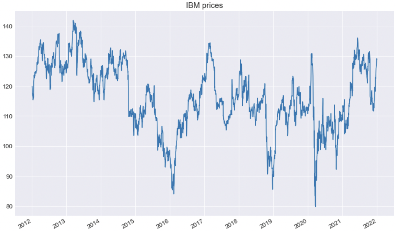
IBM returns
The following plots show the return over the 10 years window as well as the corresponding sample distribution:
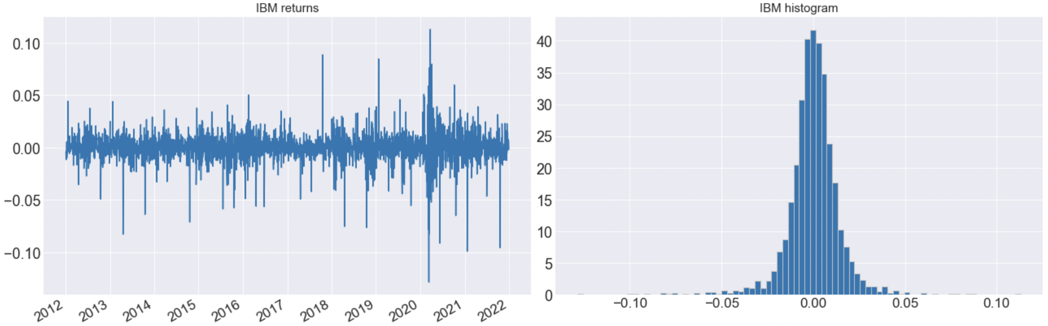
The four moments of this data, i.e., the mean, the standard deviation, the skewness, and the kurtosis are about 0.01%, 1.44%, -0.64, and 11.12, respectively. In particular, a skewness of -0.64 means that the distribution is slightly shifted to the right whereas the kurtosis of about 11 means that the tails are pretty large (given that a standard normal distribution has a kurtosis equal to 3).
This is already a first thing sugggesting the not normality of our return series. A second way to convince ourself, before proceeding with the hypothesis testing is by looking at the Q-Q plot.
In a Q-Q plot, the x-axis displays the theoretical quantiles of a standard normal distribution. That is, it represents where our data would be if they were normally distributed. On the other hand, the y-axis displays our actual data. This means that if the data values fall aproximately along the straight line then the data is normally distributed.
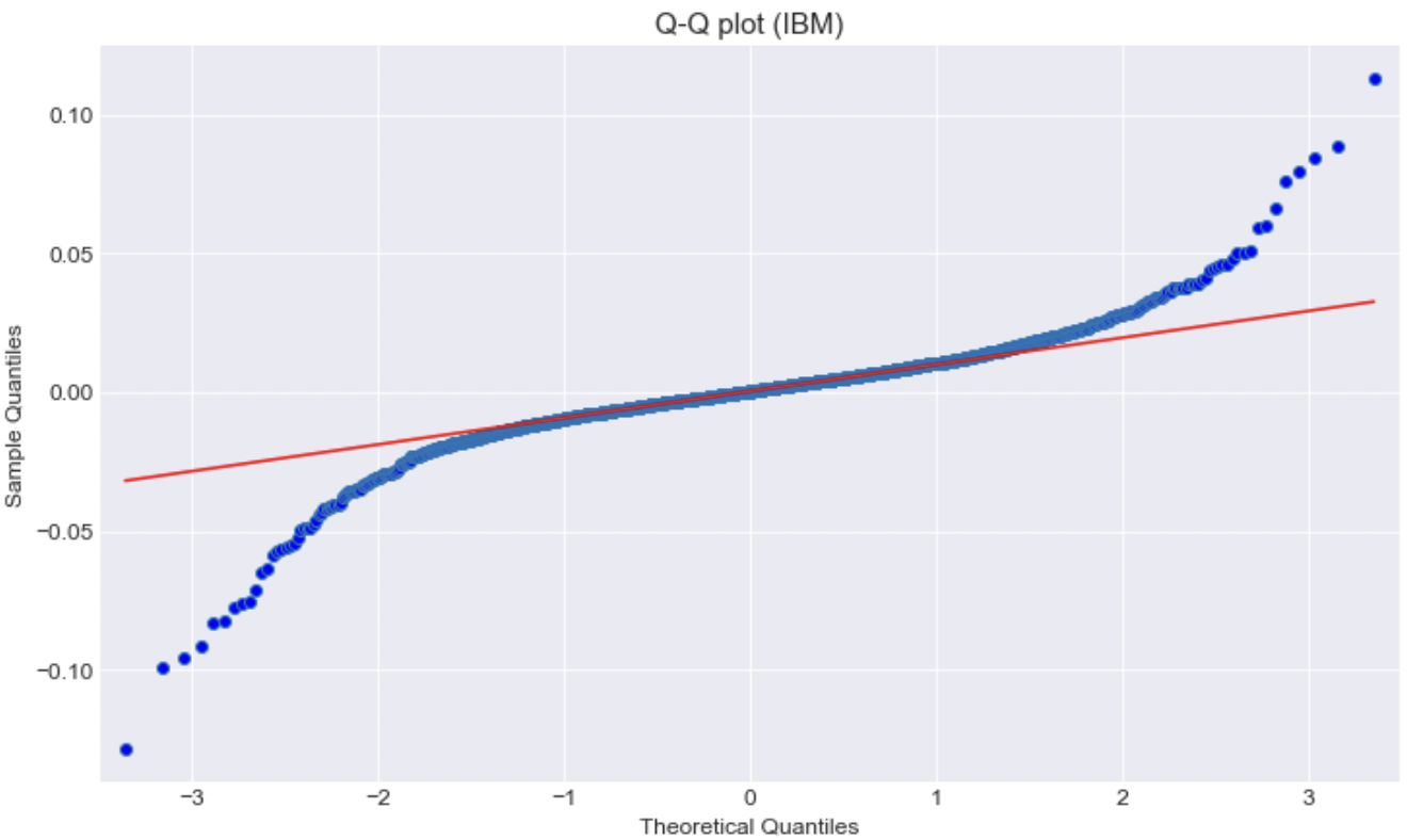
It goes without saying that this is not the case. Our returns are definitively not normally distributed. Moreover, the large deviations on the tails evidence that they are indeed fatter that the tails of a normal distribution.
Therefore, suppose that our hypothesis is that the distribution is a t-Student one:
- $H_0 = $ IBM returns are t-Student distributed.
- $H_1 = $ IBM returns are not t-Student distributed.
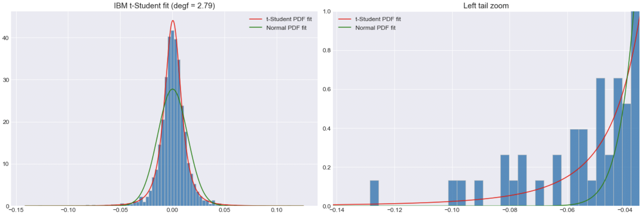
The best t-Student fit is a distribution with mean, standard deviation, and degrees of freedom equal to about 0.04%, 0.8%, and 2.79, respectively. The plots also show a normal distribution fit. Overall, it can be seen how the continuous t-Student distribution is much more closer to the sample data.
Hypothesis testing on IBM returns
Even though the distribution of the returns is clear, let us perform the hypothesis testing on the fitted t-Student distribution. As described previously, given the two test statistics KS and AD, we need to find the critical values relating to our hypothesized $F_H$ distribution.
That is, let $F_E$ be the ECDF of the sample return series. Let $F_H$ be the fitted t-Student distribution with 2.79 degress of freedom. We run the Monte Carlo simulation described beforehand:
import pandas as pd
import numpy as np
from scipy import stats
from statsmodels.distributions.empirical_distribution import ECDF

def mc_test_stats(FH, size=1000, mcsamples=1000, dtype="t"):
    KS = []
    AD = []
    for k in range(mcsamples):
        if dtype == "t":
            # STEP 1, 2, and 3: simulate a new sample given the t-Student FH distribution
            u = np.random.random(size=size)
            sample = pd.Series( stats.t(df=FH["degf"], loc=FH["mu"], scale=FH["sigma"]).ppf(u) )

            # STEP 4: fit the new sample via MLE
            df, mu, std = stats.t.fit(sample)
            FH_hat = pd.Series(np.sort( stats.t.cdf(sample, df=df, loc=mu, scale=std)), index=np.sort(sample))

        elif dtype == "n":
            # STEP 1, 2, and 3: simulate a new sample given the t-Student F_H distribution
            u = np.random.random(size=size)
            sample = pd.Series( stats.norm(loc=FH["mu"], scale=FH["sigma"]).ppf(u) )

            # STEP 4: fit the new sample via MLE
            mu, std = stats.norm.fit(sample)
            FH_hat = pd.Series(np.sort( stats.norm.cdf(sample, loc=mu, scale=std)), index=np.sort(sample))

        # STEP 5: computing the ECDF of the sample
        FE_hat = ECDF(sample)
        FE_hat = pd.Series(FE_hat.y, index=FE_hat.x)
        FE_hat = FE_hat.drop(index=FE_hat.index[0])

        # STEP 6: computing the test statistic (KS and AD)
        KS.append( max( abs(FE_hat - FH_hat) ) )
        AD.append( max( abs(FE_hat - FH_hat).divide(np.sqrt(FH_hat.multiply(1 - FH_hat))) ) )

        # STEP 7: the loop is repeated "mcsamples" times

    KS = pd.Series(KS)
    AD = pd.Series(AD)

    return KS, AD
By choosing a significance level of 5%, the critical values are then computed as the 5-th quantile of the KS and AD sample distribution:
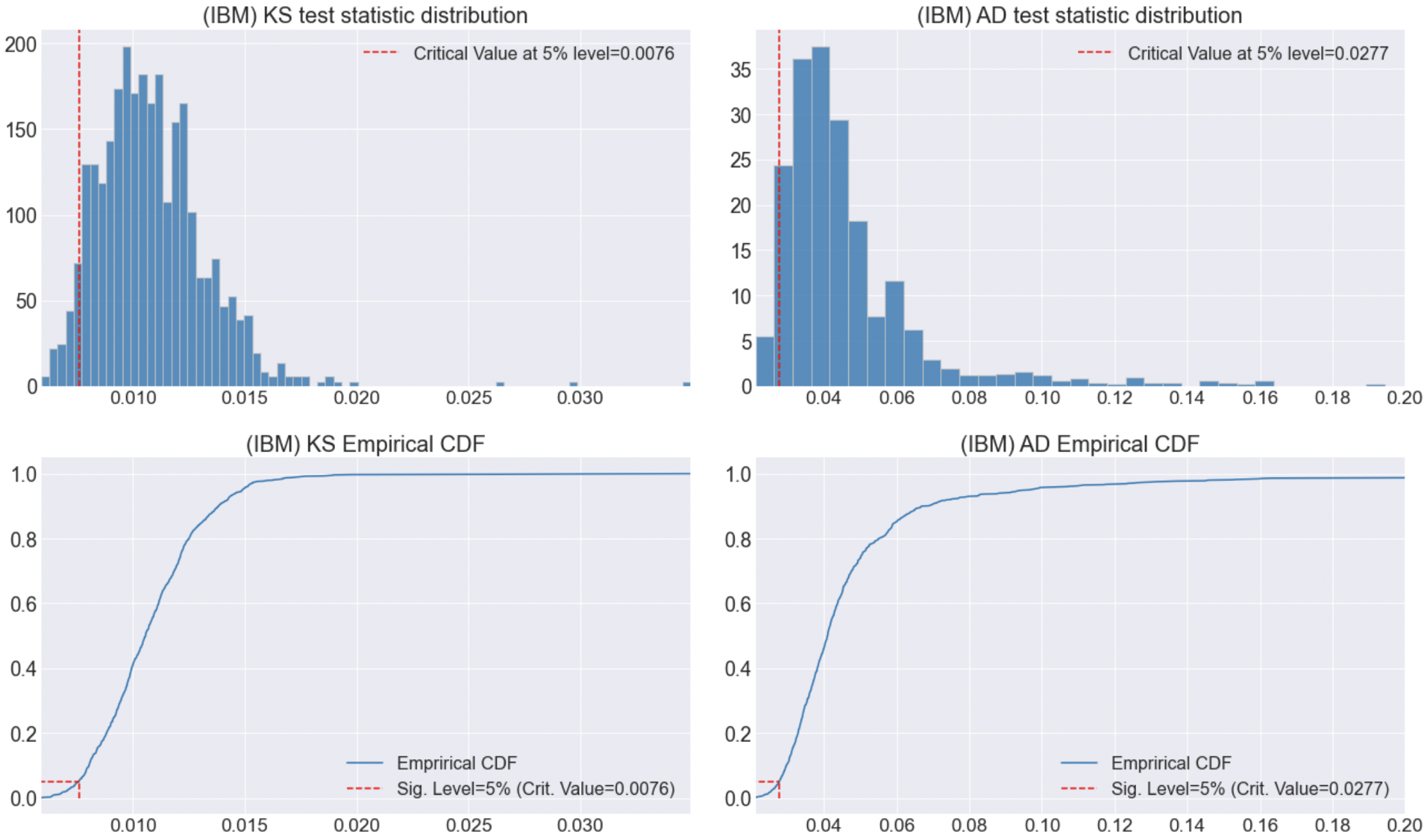
Since we now have the critical values of the KS and AD test stastic for our hypothesized distribution we are left to the hypothesis and make a decision.
To do so, given the ECDF $F_E$ of the return series, the corresponding hypothesized t-Student distribution $F_H$, we now compute both the KS and AD test statistics.
import pandas as pd
import numpy as np
from scipy import stats
from statsmodels.distributions.empirical_distribution import ECDF

def get_empirical_cdf(data):
    FE = ECDF(data)
    FE = pd.Series(FE.y, index=FE.x, name="Emprirical CDF")
    FE = FE.drop(index=FE.index[0])
    return FE

def get_hypothetical_cdf(data, FH, distype = "t"):
    if distype == "n":
        return pd.Series(np.sort(stats.norm.cdf(data, loc=FH["mu"], scale=FH["sigma"])),
                         index=np.sort(data),
                         name="Hypothesized Normal")
    elif distype == "t":
        return pd.Series(np.sort(stats.t.cdf(data, df=FH["degf"], loc=FH["mu"], scale=FH["sigma"])),
                         index=np.sort(data),
                         name="Hypothesized t-Student")

def test(FE, FH, testype="KS"):
    if testype == "KS":
        return max(abs( FE - FH ) )
    elif testype == "AD":
        return max(abs( FE - FH ).divide( np.sqrt(FH.multiply(1 - FH)) ) )

def pvalues(teststat, critval):
    return ECDF(teststat)(critval)


# FE and # FH
FE = get_empirical_cdf(rets)
FH = get_hypothetical_cdf(rets, tdist, dtype="t")

# Critical values
test_KS = test(FE, FH, testype="KS")
test_AD = test(FE, FH, testype="AD")

# p-values
pvalue_KS = pvalues(KS, test_KS)
pvalue_AD = pvalues(AD, test_AD)
If we print out test_KS and test_AD we get 0.089 and 0.0431, respectively. The corresponding p-values given the KS and the AD distributions are about 21% and 58%, respectively.
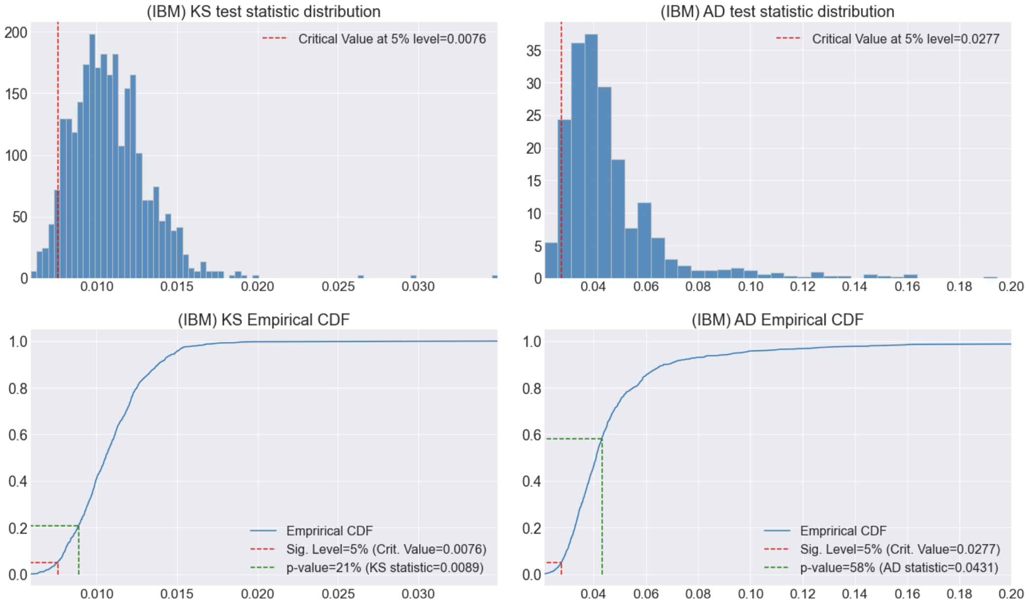
Since both p-values are above the significance level of 5% (or, in other words, the corresponding test statistics computed of 0.089 and 0.0431 are larger than the critical values 0.0076 and 0.0277, respectively) we have not enough evidence to reject the Null Hypothesis.
In conclusion, the Null Hypothesis is accepted, i.e., IBM returns are t-Student distributed.