Fixed-Income instruments: Bond pricing – Quant Finance
29 June 2022A bond is a type of a fixed-income instrument that essentially represents a loan made by some investor to a borrower. Bonds are used by companies, municipalities, and sovereign governments to finance projects/operations. The owners of bonds are called bondholders, or simply lenders, since they are the ones that lend money and obtain the bond.
As any other financial contract, once issued, bonds are tradable assets. Many corporate and government bonds are publicly traded. Others are traded only over-the-counter (OTC) or privately between the borrower and lender.
They are fixed-income instruments since they tradionally pay a fixed interest rate (in form of coupons) to the debtholder. This interest is paid by the corresponding borrower.
In this post we will see several things, for example, how to price a bond or how to build yield curves with a method called bootstrap.
Main characteristics of bonds
There are some common basic characteristics that are shared by most type of bonds
-
Face (Par) Value. This is the amount of money the bond will be worth when expiries. It is typically set to $\$1000$ or $\$100$.
- If the bond price is less than the Face Value, then the bond is said to be trading at discount.
- If the bond price is higher than the Face Value, then the bond is said to trading at premium.
- Coupon rate: It is the rate of interest the borrower pays with respect to the face value of the bond, expressed as a percentage. For instance, a $5\%$ annual coupon rate means that bondholders will receive $\$50 = 5\% \cdot \$1,000$ every year.
- Coupon dates. These are fixed dates on which the borrower pays interests (i.e., when bondholders receive the coupons). Such payments can be made at any interval, although standard intervals are annual (e.g., for Spanish bonds) or semiannual (e.g. for Italian bonds) payments.
- Maturity date. This is the date on which the bond expiries and the borrower will re-pay the bondholders the face value of the bond (as well as the last coupon).
Zero-Coupon bonds and Zero-Rates
Amongst all different types of bonds, the most simple one is the so called zero-coupon bond which, as the name says, it does not pay any coupon. It rather pays the bond's face value plus a fixed interest in just one payment on the expiration date. For example, US Treasury bills are a zero-coupon bonds.
With such a type of bond, if the maturity is in $n$ years, the bondholder' interest and principal are realized only at the end of $n$-th year. In this context, the $n$-year zero-coupon interest rate is sometimes referred to as the $n$-year spot rate or zero rate.
For example, suppose that a bond with maturity 5 years pays a zero-rate of 3% per annum. With continuous compounding, this means that if one invest $\$100$ today, then at the end of the 5-th years, we would have: $$ \$100 \cdot e^{0.03\cdot 5} = \$116.2 $$ Note that the majority of interest rates observed in the marked are not pure zero-rates. In fact, if we have a 5-year government bond with some coupon rate, the price of such bond does not determine the 5-year zero-rate because some of the interest will be paid in form of coupons during the life of the bond. We will come back to this point later.
Now, given that the interest plus the face value is obtained at maturity, the bond today should be worth the discounted value of such expected quantity.
These bonds are then generally sold at discount, in order to match the face value at maturity. That is, given the same $5$-year bond with a zero-rate of 3% annum, the bond price will be $$ B = 100 \cdot e^{-0.03 \cdot 5} = \$86.07. $$
Coupon-bearing bond pricing
What is the price of a coupon-bearing bonds?
Differently from the zero-coupon bond, in which we had only one unique cash-flow to discount, now we have to take into account all periodic coupon payments. However, the pricing method is the same.
The bond price in this case will be simple given by the sum of all discounted cash-flow payments. These payments will be coupons during the entire life of the bond and the coupon plus the face value at maturity.
- 1% zero-rate at 0.5 years.
- 1.2% zero-rate at 1 year.
- 2.5% zero-rate at 1.5 years.
- 3.1% zero-rate at 2 years.
Given a face value of $\$100$, we will receive the first coupon of $\$1 = (2\%/2) \cdot \$100$ after 6 months (half coupon is paid after half year). Then, another $1\$$ at the end of the 1st year. Then, $1\$$ after 1.5 years. Finally, we will receive $\$101 = (2\%/2) \cdot \$100 + \$100$ at the end of the 2nd year.
Then, we just need to discount these cash-flow payments using the corresponding given zero-rates. That is
- A first $\$$1 discounted at 1% rate for the first 0.5 years.
- Then, $\$$1 discounted at 1.2% rate for 1 year.
- Another $\$$1 discounted at 2.5% rate for 1.5 years.
- Finally, $\$$101 discounted at 3.1% rate for 2 years.
Yield-to-Maturity
The Yield-to-Maturity (YTM) is the single discount rate that, when applied to all cash-flows gives a theoretical bond price equal to its market price.
Recall that in the previous example we have discounted each cash-flow using the associated interest rate for the time at which the payment occur (because we have been provided a term-structure curve).
However, suppose that the theoretical bond price computed, $B = \$97.87$, is also the current market value. Now, if we let $y$ be the single rate such that the bond price is obtained, we would have that: $$ B = 1\cdot e^{-y\cdot 0.5} + 1\cdot e^{-y\cdot 1} + 1\cdot e^{-y\cdot 1.5} + 101\cdot e^{-y\cdot 2} = \$97.87. $$ Then, by solving the equation we would find the YTM of the bond.
This can be solved using some iterative trial and error procedure. For example, the Newton-Raphson method. In fact, the problem here is to find the zero of a given function. Let $$ F(y) := c \sum_{i=1}^{n-1} e^{-y t_i} + (c+F)e^{-y t_n} - B , $$ where $y$ is our unknown YTM and $B$ is the theoretical (market) price of the bond. We seek the value of $y$ such that $F(y) = 0$. Let $$ F'(y) = -c \sum_{i=1}^{n-1} t_i e^{-y t_i} - (c+F)t_n e^{-y t_n} , $$ be the first derivative in $y$. The Newton-Raphson method iteratively finds the root by updating the guess as follows $$ y_{k+1} = y_k - \frac{F(y_k)}{F'(y_k)} , $$ where $y_0$ is a starting initial guess for $y$.
The following python functions will do the job:
def bond_ytm(fvalue   = 100,
             price    = 97,
             time     = [0.5, 1, 1.5, 2],
             cashflow = [1, 1, 1, 101],
             tol      = 1e-8,
             y0       = 0.10,
             maxiter  = 100):
    '''
    Newton-Rapson method for Bond's Yield-to-Maturity calculation
    '''
    # F(y)
    F  = lambda y: sum( [chf * np.exp(-y * t) for chf, t in zip(cashflow, time)] ) - price

    # Derivative F'(y)
    dF = lambda y: sum( [ -chf * t * np.exp(-y * t) for chf, t in zip(cashflow, time)] )

    # Error due to first guess
    err = F(y0)

    # Iterative loop
    ii = 0
    while abs(err) > tol:
        # Compute new point
        ynew = y0 - F(y0) / dF(y0)
        # Compute the current error
        err = F(ynew)
        # Update the current guess
        y0 = ynew
        # Check maximum iterations
        ii = ii + 1
        if ii == maxiter:
            print("Max. iteration reached")
            return y0

    return y0
The YTM for our data is about $y = 3.0828\%$.
Note that there is an inverse relationship between the bond price and its yield-to-maturity. Since the formula is: $$ B = c \sum_{i=1}^{n-1} e^{-y t_i} + (c+F)e^{-y t_n}, $$ when $y$ increases, then $B$ decreases, and vice versa. If we plot the bond price against the YTM we would get this:
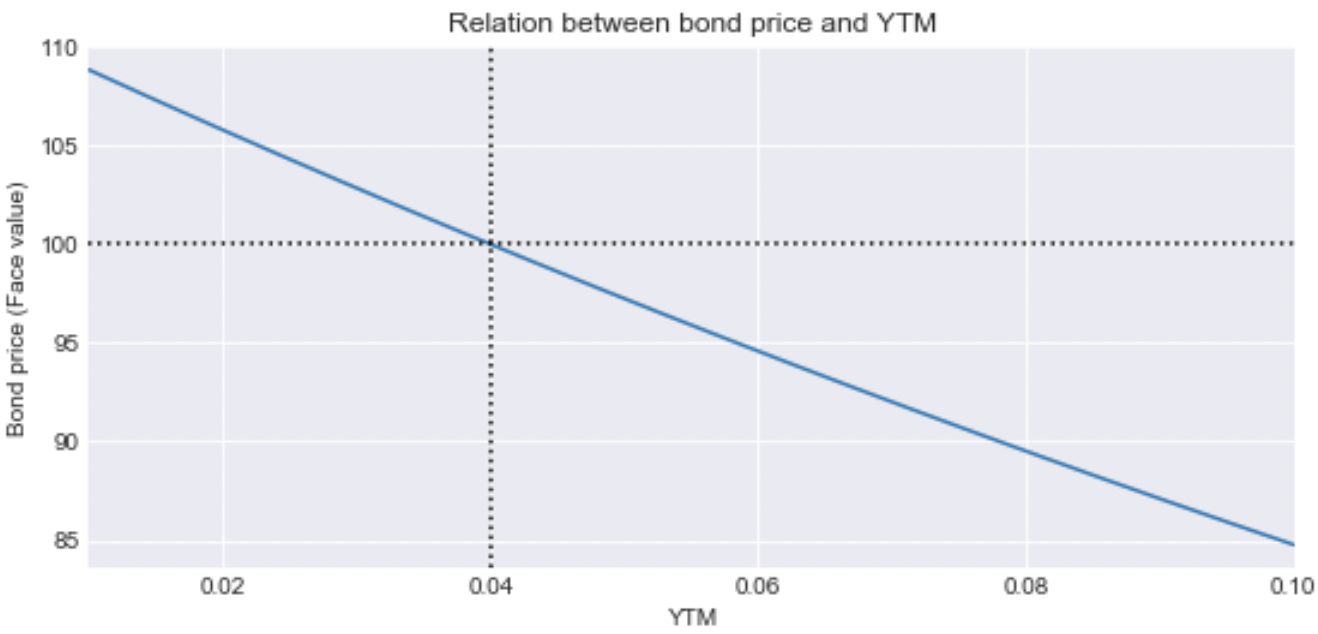
We could have deduced this by the first derivatives $F'(y)$ we saw beforehand. It is negative. In particular:
- The bond will trade at discount (bond price < face value) when the YTM is larger than the coupon rate.
- The bond will trade at premium (bond price > face value) when the YTM is smaller than the coupon rate.
Par Yield
The Par Yield for a certain bond maturity is that coupon rate such that the bond price equals its face value.
That is, we first need to look for the coupon payment $c$ such that: $$ B = c \sum_{i=1}^{n-1} e^{-r_i t_i} + (c+F) e^{-r_n t_n} = F $$ This is solved by: $$ B = c \sum_{i=1}^{n} e^{-r_i t_i} + Fe^{-r_n t_n} = F \quad\Longrightarrow\quad c = \frac{F(1 - e^{-r_n t_n})}{ \sum_{i=1}^{n} e^{-r_i t_i} } . $$ If we use the same zero-rates introduced beforehand, we get: $$ c = \frac{100\cdot(1 - e^{-0.031\cdot 2})}{ e^{-0.01\cdot 0.5} + e^{-0.012\cdot 1} + e^{-0.025\cdot 1.5} + e^{-0.031\cdot 2}} \approx \$1.546 $$ Note that in our example the coupon was paid semiannually. Then, we have indeed found the semiannual coupon. The annual one is therefore $\$$2.546.
Bond Duration
The Duration of a bond is a measure of how long on average the bondholder has to wait before receiving all cash payments. It is also called Macaulay Duration, from Frederick Macaulay who introduced it in 1938.
For example, a zero-coupon bond that lasts $n$ years has a duration of just $n$ years since there are no intermediate cash-flows. Then, the time waited to get the (only) payment is exactly $n$ years.
However, a coupon-bearing bond lasting $n$ years has a duration of something less than $n$ years, because the bondholder receives cash-flows in terms of coupons prior to the $n$-th year.
Recall that the price of a coupon-bearing bond is $$ B = \sum_{i=1}^n C_i e^{-r_i t_i} , $$ where $C_i = c$ for $i=1,\dots,n-1$ are the coupon payments and $C_n=c + F$ is the last coupon plus the face value of the bond. That is, the bond price is nothing but that the sum of the present values of all bond's cash-flows.
The bond Duration is defined as follows: $$ D := \frac{ \sum_{i=1}^n t_i C_i e^{-r_i t_i} }{B} = \sum_{i=1}^n t_i \left(\frac{ C_i e^{-r_i t_i} }{ B }\right) = \sum_{i=1}^n t_i \left(\frac{ C_i e^{-r_i t_i} }{ \sum_{k=1}^n C_k e^{-r_k t_k} }\right) . $$ The term in brackets is the ratio of the present value of the cash-flow at time $t_i$ to the bond price. Therefore, the Duration is a weighted average of the times when payments are made, with the weight applied to time $t_i$ being equal to the proportion of the bond’s total present value provided by the cash flow at time $t_i$.
Note that here all discounting are done using zero-rates $r_i$ for each time $t_i$. However, we can also simply discounting by using a fixed YTM $y$ as follows: $$ D = \sum_{i=1}^n t_i \left(\frac{ C_i e^{-y t_i} }{ \sum_{k=1}^n C_k e^{-y t_k} }\right) . $$
The Duration is an important quantity for the following reason. A first-order approximation of $\Delta B$ is given by (see Taylor expansion): $$ \Delta B = \frac{dB}{dy} \Delta y = \frac{d}{dy}\left( \sum_{i=1}^n C_i e^{-y t_i} \right) \Delta y = - \sum_{i=1}^n t_i C_i e^{-y t_i} \; \Delta y $$ Therefore, from the definition of Duration $D$ we get: $$ \frac{\Delta B}{B} = - \frac{ \sum_{i=1}^n t_i C_i e^{-y t_i} }{B} \; \Delta y = - D \Delta y \qquad\text{that is}\qquad \Delta B = - B D \Delta y . $$ We then have a formal relation between the change in bond price and the change in the corresponding bond YTM (note the inverse relationship we have already seen before).
Let us compute the Duration of the bond we have considered so far, i.e., the $2$-years bond with a coupon rate of 2% per annum paid semiannually. For a face value $F=100$, this bond pays $\$1$ every six months. Also, recall that the corresponding YTM was $y=3.0828\%$ and that the bond price was $\$97.87$.
Then, to compute the Duration, we first compute the present values of the cash-flows. For example, the present value of the first coupon payment is $C_1\cdot e^{-y t_1} = 1\cdot e^{-0.030828 \cdot 0.5} = 0.985$. The corresponding weigth is then given by this amount over the bond price, i.e., $0.985 / 97.87 = 0.010$. Finally, this weigth is multiplied by the time $t_1$, $ 0.010 \cdot 0.5 = 0.005$.
If we keep computing until the 2nd year, we will get the following results:
| Time (years) | Cash-flows ($) | Present Value | Weigth | Time $\cdot$ Weigth |
|---|---|---|---|---|
| 0.5 | 1 | 0.985 | 0.010 | 0.005 |
| 1 | 1 | 0.9696 | 0.0099 | 0.0099 |
| 1.5 | 1 | 0.9548 | 0.0098 | 0.0146 |
| 2 | 101 | 94.9608 | 0.9703 | 1.9406 |
Note that if we sum the values in the Present Value columns, they sum to the bond price $\$97.87$. On the other hand, the bond Duration is given by the sum of the last columns Time $\cdot$ Weigth. This is equal to 1.97 years.
Once we have the Duration of our bond, we can now check how accurate is the estimate of the $\Delta B$ is computed by using the Price-Yield relation. In fact, we would have that: $$ \Delta B = - B D \Delta y = - 97.87 \cdot 1.97 \cdot \Delta y = -192.82 \cdot \Delta y. $$ Now, suppose that the YTM of the bond decreases by 5 basis points. This is equal to $\Delta y = -0.05\%$. Then, the relationship predicts $\Delta B = -192.82 \cdot (-0.0005) = +0.09641$, that is the new bond price will be $$ 97.87 + 0.09641 = \$97.96641. $$
In order to see how accurate is this we should re-calculate the new bond price with the new yield. That is, given the new YTM $y = 3.0828\% - 0.05\% = 3.0328\%$, we have: $$ B = 1\cdot e^{-0.030328\cdot 0.5} + 1\cdot e^{-0.030328\cdot 1} + 1\cdot e^{-0.030328\cdot 1.5} + 101\cdot e^{-0.030328\cdot 2} = \$97.96645. $$ Well, this is accurate up to the fourth decimal point in this case.
Yield Curve: the Bootstrap method
Let us conclude the post by describing a very common method used by financial firms to determine the zero-rates (hence, to construct the so called yield curve) called the bootstrap method.
The method calculates the zero-rates by using the market prices of bonds and using the theoretical bond pricing formulas. Consider the bond's data in the following table:
| Face Value ($) | Maturity (years) | Coupon Rate (%) | Price ($) |
|---|---|---|---|
| 100 | 0.25 | 0 | 97.52 |
| 100 | 0.50 | 0 | 94.12 |
| 100 | 1.00 | 2 | 89.78 |
| 100 | 1.50 | 8 | 92.10 |
| 100 | 2.00 | 12 | 95.50 |
Assume that the first two bonds a re zero-coupon bonds (coupn rate equal to 0), whereas the last three bonds are coupon-bearing and coupons are per annum, paid semiannually every six months.
We start from the lowest maturity. For the first zero-coupon bond, we know that the current market price of $\$97.52$ will be the face value of $\$100$ within 0.25 years. That is, $100 = 97.52\cdot e^{r_{0.25} \cdot 0.25}$. From this, we recover $r_{0.25}$: $$ r_{0.25} = \log( 100 / 97.52 ) / 0.25 = 10.045\%. $$
The zero-rate for 0.5 years can be found in the same way using data for the second zero-copuon bond. We know that $100 = 94.12\cdot e^{r_{0.50} \cdot 0.50}$. Then: $$ r_{0.50} = \log( 100 / 94.12 ) / 0.50 = 12.120\%. $$
For the zero-rate corresponding to 1 year, we now use the data of the third bond, which is a coupon-bearing bond. Then, we know that the price of this bond is given by the sum of the cash-flows discounted with corresponding zero-rate according to payment dates.
Since the coupon rate is 2% per annum paid semiannually, the bond will pay $\$1$ on 0.5 years and after 1 year. Therefore, to compute the zero-rate $r_{1}$ we will use the zero-rate $r_{0.50}$ we have just computed. The bond price will be given by: $$ 1\cdot e^{-0.12120 \cdot 0.5} + 101\cdot e^{-r_1 \cdot 1} = 89.78. $$ This gives: $$ r_1 = -\frac{1}{1} \log\left( \frac{89.78 - 1\cdot e^{-0.12120 \cdot 0.5}}{101} \right) = 12.830\% . $$
So far, we have found the zero-rates $r_{0.25}$, $r_{0.50}$, and $r_1$. Given now the coupon bearing bond for 1.5 years we use the same method to recover the zero-rate $r_{1.5}$: $$ 4\cdot e^{-0.12120 \cdot 0.5} + 4\cdot e^{-0.12830 \cdot 1} + 104\cdot e^{-r_{1.5} \cdot 1.5} = 92.10. $$ Solving for $r_{1.5}$ gives $r_{1.5} = 13.593\%$.Finally, we can find the last zero-rate $r_2$ by imposing: $$ 6\cdot e^{-0.12120 \cdot 0.5} + 6\cdot e^{-0.12830 \cdot 1} + 6\cdot e^{-0.13593 \cdot 1.5} + 106\cdot e^{-r_{2} \cdot 2} = 95.50. $$ This gives $r_{2} = 14.27\%$.
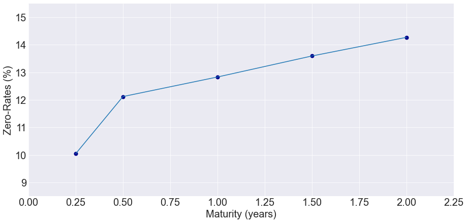
Therefore, we ended up the following yield curve:
| Maturity (years) | Zero-Rate (%) |
|---|---|
| 0.25 | 10.045 |
| 0.50 | 12.120 |
| 1.0 | 12.830 |
| 1.5 | 13.593 |
| 2.0 | 14.270 |
The following figure shows the computed yield curve: