The log-normal property of stock prices – Quant Finance
10 November 2021The log-normal property of stock prices is a fundamental assumption of the Black-Scholes option pricing model.
Although the model makes several assumptions (e.g., it is assumed that volatility is constant), a very important one is that stock prices follow a log-normal distribution.
In turn, this means that stocks' log-returns are normally distributed.
Let $S_t$ be the price of a stock at time $t$ and suppose that it follows the following Stochastic Differential Equation $$ dS_t = a\,dt + b\, dB_t , $$ where $$ a=a(S_t,t):=\mu S_t \qquad\text{and}\qquad b=b(S_t,t):=\sigma S_t. $$ This is referred to as Generalized Brownian Motions (GBM) and we talked about it in this post. Here, $a$ is called the drift rate of the motion whereas $b^2$ is the corresponding variance rate.
In particular, when both the drift and the variance rates depend on an underlying variable (in this case, $S_t$) and time $t$, the process is referred to as Itô process.
For every $t\geq 0$, define the following logarithm of the stock price: $$ \label{eq:logS} F_t = F(S_t, t) := \ln(S_t). $$
Distribution of the logarithm of stock prices using Itô's Lemma
First of all, let us recall what Itô's Lemma states:
A (not so rigorous) proof of Itô's Lemma can be found here.
Our function $F_t$ defined as the logarithm of the stock price is a continuous and differentiable functions of $S_t$ and $t$. We can then apply Itô's Lemma where $x = S_t$.
We have to compute the following components $\frac{\partial F}{\partial t}$, $\frac{\partial F}{\partial S_t}$, and $\frac{\partial^2 F}{\partial S_t^2}$. We get: \begin{align*} \frac{\partial F}{\partial t} &= \frac{\partial}{\partial t}\ln(S_t) = 0, \\[6pt] \frac{\partial F}{\partial S_t} &= \frac{\partial}{\partial S_t}\ln(S_t) = \frac{1}{S_t}, \\[6pt] \frac{\partial^2 F}{\partial S_t^2} &= \frac{\partial}{\partial S_t}\left(\frac{\partial}{\partial S_t}\ln(S_t)\right) = \frac{\partial}{\partial S_t}\left(\frac{1}{S_t}\right) = -\frac{1}{S_t^2}. \end{align*} Given that $a=\mu S_t$ and $b=\sigma S_t$, substituing into Itô's Lemma, we obtain: $$ \label{eq:path:lognorm} dF_t = \left(\frac{1}{S_t}\mu S_t - \frac{1}{2}\frac{1}{S_t^2}\sigma^2 S^2_t\right)dt + \frac{1}{S_t}\sigma S_t dB_t = \left(\mu -\frac{\sigma^2}{2}\right)dt + \sigma dB_t. $$ Since $\mu$ and $\sigma$ are constants, this equation shows that the logarithm of stock prices, $F_t=\ln(S_t)$, follows a Generalized Brownian Motion with drift rate equal to $\mu-\sigma^2/2$ and variance rate equal to $\sigma^2$.
Therefore, since $$ dF_t = F_{t+dt} - F_t = \ln(S_{t+dt}) - \ln(S_t) = \ln\left(\frac{S_{t+dt}}{S_t}\right), $$ by definition of Brownian Motion, we have that stock prices' log-returns are normally distributed with mean $(\mu-\sigma^2/2)dt$ and variance $\sigma^2dt$, i.e., $$ \ln\left(\frac{S_{t+dt}}{S_t}\right) \sim \mathcal{N}\left(\left(\mu-\frac{\sigma^2}{2}\right)dt,\sigma^2dt \right). $$ Note that this is indeed equivalent to $$ \label{eq:logprice:normal} \ln(S_{t+dt}) \sim \mathcal{N}\left(\ln{S_t} + \left(\mu-\frac{\sigma^2}{2}\right)dt,\sigma^2dt \right). $$ which means that the logarithms of stock prices are normally distributed. Due to the definition of lognormal random variables, this implies that stock prices are log-normally distributed.
By the properties of the lognormal distribution, it can be shown that the mean of $S_t$, for all $t\geq 0$, is $$ \label{eq:mean:lognormal} \mathbb{E}(S_t) = S_0e^{\mu t}. $$ This is a result used to derive the Black-Scholes option pricing model.
Distribution of the logarithm of stock prices without using Itô's Lemma
Let us recover the equation describing the (Brownian) motion for the logarithm of stock prices without explicitly using Itô's Lemma.
First of all, note that if $S_t$ follows an Itô process with $dB_t$ being a Brownian Motion, we can write $dB_t = \xi \sqrt{dt}$, where $\xi\sim\mathcal{N}(0,1)$, and: $$ d S_{t} = \mu S_t dt - \sigma S_t \xi \sqrt{dt} \quad\Longrightarrow\quad \frac{d S_{t}}{S_t} = \mu dt - \sigma \xi \sqrt{dt}. $$ Furthermore, for any small real $x$, note that $$ \label{eq:pro:log} \ln(1+x) \approx x - \frac{1}{2}x^2, $$ if we ignore higher order terms (this is the corresponding Taylor expansion truncated at second-order terms).
Recall that $dS_t=S_{t+dt}-S_t$. By using the results above, we can write $$ \label{eq:path:lognorm:2} \begin{split} \ln\left(\frac{S_{t+dt}}{S_t}\right) = \ln\left(1 + \frac{dS_t}{S_t}\right) &\approx \frac{dS_t}{S_t} - \frac{1}{2}\left(\frac{dS_t}{S_t}\right)^2 \\ &= \mu \,dt + \sigma\xi\sqrt{dt} - \frac{1}{2}\left(\mu\,dt+\sigma\xi\sqrt{dt}\right)^2 \\ &= \mu \,dt + \sigma\xi\sqrt{dt} - \frac{1}{2}\left(\mu^2 \underbrace{dt^2}_{\approx 0} + \sigma^2 \underbrace{dt \xi^2}_{\approx dt\mathbb{E}(\xi^2)=dt} + 2\mu \underbrace{dt \sqrt{dt}}_{\approx 0} \sigma \xi \right) \\ &\approx \mu \,dt + \sigma\xi\sqrt{dt} - \frac{1}{2}\sigma^2 dt \\ &= \left(\mu -\frac{\sigma^2}{2}\right)dt + \sigma\xi\sqrt{dt} = \left(\mu -\frac{\sigma^2}{2}\right)dt + \sigma dB_t. \end{split} $$
Analytical solution of the Geometric Brownian Motion
Let us derive the solution to the Geometric Brownian Motions followed by stock prices. So far, we have found that $$ \ln\left(\frac{S_{t+dt}}{S_t}\right) = \left(\mu -\frac{\sigma^2}{2}\right)dt + \sigma dB_t = \left(\mu -\frac{\sigma^2}{2}\right)dt + \sigma \xi\sqrt{dt}, $$ where $\xi\sim\mathcal{N}(0,1)$. Take the exponential on both sides of the equation, $$ S_{t+dt} = S_t \exp{\left( \left(\mu-\frac{\sigma^2}{2}\right)dt + \sigma\xi\sqrt{dt} \right)}. $$ Then, for every time $t = ndt$, where $n\in\mathbb{N}$, we have $$ \label{eq:sol:stock:price} \begin{split} S_t = S_{0+ndt} = S_0 \exp\left( \left(\mu - \frac{\sigma^2}{2}\right) (ndt) + \sigma\xi\sqrt{ndt} \right) &= S_0 \exp\left( \left(\mu - \frac{\sigma^2}{2}\right)t + \sigma\xi\sqrt{t} \right). \end{split} $$ This equation shows how to obtain the value of the stock price at any time positive $t\geq 0$, starting from an initial price of $S_0$.
Some of the arguments for using GBM to model stock prices are the following:
- The expected returns of GBM are independent of the value of the process (stock price), which agrees with what we would expect in reality;
- The GBM process only assumes positive values, as real stock prices do (in principle, negative stock prices are a non-sense as it is assumed that when the price goes to zero the stock is worthless and the company defaults);
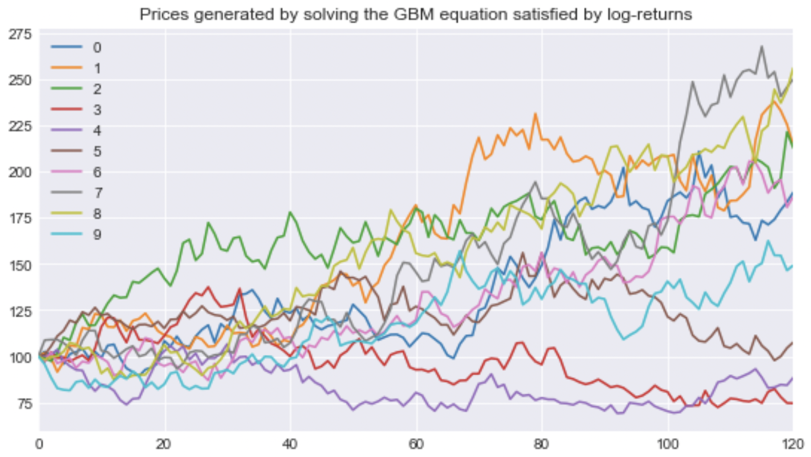
- The GBM process shows the same kind of roughness in its paths as we see in real stock price paths;
- Calculations with GBM processes are relatively easy.
- GBM processes assume a constant volatility although, in real stock price processes, the volatility changes over time (possibly stochastically);
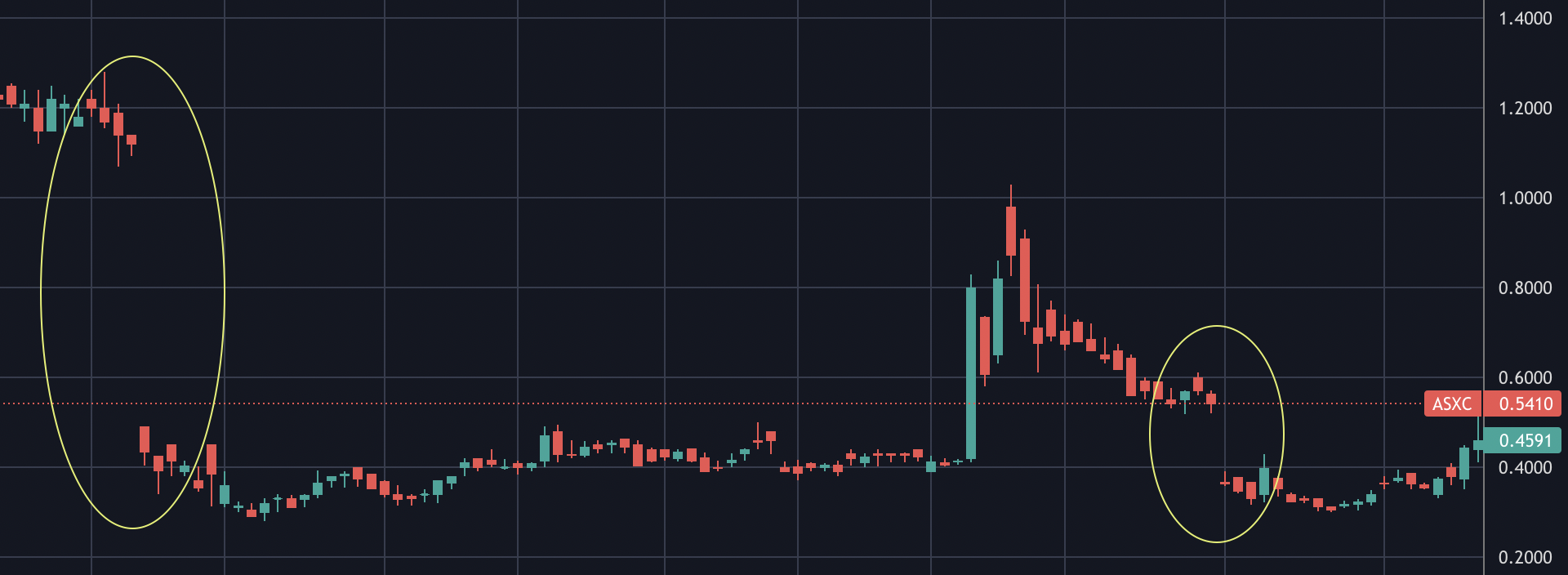
- Real stock price processes often show jumps whereas in GBM processes the path must be continuous.
For example, regarding this last point, the GBM processes are something like this:
even if real stock prices can go like this: