
Modern Portfolio Theory - Part 1 – Quant Finance
20 December 2021The Modern Portfolio Theory (MPT) is a mathematical framework that helps investors in assembling portfolios of assets such that the expected return is maximized for a certain given level of volatility.
Since its introduction by Henry Markowitz in 1952, the MPT has become a key tool for asset managers and robo-advisors alike, typically applied with a buy-and-hold strategy.
It is a formalization of diversification in investing, that is, the idea that owning different kinds of financial assets (with a certain correlation) is less risky than owning one single asset. In practice, we have to construct a portfolio of different stocks and we want to find the optimal percentages of investment to be allocated in the stocks so that, for example, the total (expected) return of such a portfolio is maximixed.
Let us formalize the problem.
Suppose we have $N > 1$ stocks and we decide to invest our capital in them. Let $\mathbf{w}:=(w_1,\dots,w_N)^T$, with $w_i\in (0,1)$ for all $i=1,\dots,N$, where each $w_i$ represents the proportion of the investiment (a percentage of the capital invested) in asset $i$. These quantities $w_i$ are the weights.
Since we invest all of our capital, there holds $\sum_{i=1}^N w_i = 1$. This is a so called long-only strategy.
Let $r_i$ and $r_p$ be the return of asset $i$ and the total return of the entire portfolio, respectively. Likewise, let $\sigma_i$ and $\sigma_p$ be the volatility of asset $i$ and the volatility of the portfolio, respectively.
Return of the portfolio
The total return of the porfolio, $r_p$, is going to be a simple weigthed average of the (total) returns of single assets, i.e., $$ r_p = \sum_{i=1}^N w_i r_i = \mathbf{w}^T \mathbf{r}, $$ where $\mathbf{r} := (r_1,\dots,r_N)^T$.
Volatility of the portfolio
The volatility of the porfolio, $\sigma_p$, is computed as the (square root of the) variance of the weigthed average of the returns of single stocks.
Let us consider an axample with only two stocks. We have two percentages $w_1$ and $w_2$ and two stocks whose returns are denoted by $r_1$ and $r_2$. We have: $$ \sigma_p^2 = \text{Var}(w_1 r_1 + w_2 r_2) = w_1^2 \text{Var}(r_1) + w_2^2\text{Var}(r_2) + 2w_1 w_2\text{Cov}(r_1,r_2) = w_1^2 \sigma_1^2 + w_2^2 \sigma_2^2 + 2 w_1 w_2\text{Cov}(r_1,r_2), $$ where $$ \text{Cov}(r_1,r_2) := \mathbb{E}[(r_1-\mu_1)(r_2 - \mu_2)], $$ is the covariance between the two stocks and where $\mu_1$ and $\mu_2$ denote their mean returns, respectively. In particular, if we denote by $$ \rho_{1,2} := \frac{\text{Cov}(r_1,r_2)}{\sigma_1 \sigma_2}, $$ the correlation coefficient between the two stocks, then the volatility of a $2$-stocks portfolio becomes: $$ \sigma_p = \sqrt{ w_1^2 \sigma_1^2 + w_2^2 \sigma_2^2 + 2w_1 w_2 \sigma_1 \sigma_2 \rho_{1,2} }. $$ Recall that a correlation equal to $1$ mean than the assets are completely correlated, whereas a correlation equal to $-1$ means thant the stocks are conversely correlated. Note that, using matrix notation, we can write in compact form such a volatility. That is: $$ \sigma_p = \sqrt{ (w_1, w_2)\, \begin{pmatrix} \sigma^2_1 & \sigma_1 \sigma_2 \rho_{12} \\ \sigma_1 \sigma_2 \rho_{21} & \sigma^2_2 \end{pmatrix} \begin{pmatrix} w_1 \\ w_2 \end{pmatrix} } = \sqrt{ \mathbf{w}^T \Sigma \mathbf{w} } \qquad\text{with}\qquad \Sigma := \begin{pmatrix} \sigma^2_1 & \sigma_1 \sigma_2 \rho_{12} \\ \sigma_1 \sigma_2 \rho_{21} & \sigma^2_2 \end{pmatrix}, $$ where $\Sigma$ is the symmetric square covariance matrix of the two stocks.
Now, in case of $N$ stocks, let again $\Sigma = [c_{ij}]$ be the $N\times N$ covariance matrix where each element $c_{ij} := \sigma_i \sigma_j \rho_{ij}$, for $i,j=1,\dots,N$, denotes the covariance between assets $i$ and asset $j$, and with $\sigma_i$, $\sigma_j$, and $\rho_{ij}$ being the volatilities and the correlation coefficients of assets $i$ and $j$, respectively. Of course, when $i=j$, $c_{ii}=\sigma_i^2$ is simply the variance of asset $i$ (these are the diagonal entries of the covariance matrix).
Therefore, the volatility of the portfolio is given by: $$ \sigma_p = \sqrt{ \mathbf{w}^T \Sigma \mathbf{w} }. $$
Efficient Frontiers
In the MPT, given the volatility-return plane, i.e., the plane in which each point denotes a portfolio with a certain (expected) return for a given fixed volatility, the efficient frontier is a curve denoting the efficient part of the plane.
That is, it is the set of portfolios constructed with a given input assets (e.g., stocks) and having the maximum expected returns for a fixed level of volatility and, in turn, the lowest volatilities for a fixed level of expected return.
Efficient Frontier of a hypothetical 2-stocks portfolio
Suppose we have a certain amount of money to invest into 2 stocks. Let us see which kind of curve, or efficient frontier, we obtain by designing 20 different portfolios by using 6 different correlations between the two stocks.
First of all, let us clarify that when we talked about the return of a stock, we mean just one single number, for example, the annualized return (or return per year). This is nothing but that the overall compound return of the stocks at the end of 1-year period (e.g., 252 sessions). Have a look here.
To do so, we first setup the following mean returns, $\mu_1 = 0.001019$, $\mu_2=0.001249$, and volatilities $\sigma_1=0.016317$, $\sigma_2=0.019129$. Then, we generate 500 daily returns for both stocks by using the following set of 6 correlations $\rho = (1, 0.6, 0.2, -0.2, -0.6, -1)$ from a multivariate gaussian distribution and using the mean returns and the corresponding covariance matrix $\Sigma$.
Once we have the set of 500 daily returns, we obtain the corresponding annualized returns $\mathbf{r} = (r_1, r_2)$. With these two numbers, we compute the returns of the 20 portfolios we can construct by allocating the weigths into the stocks, $r_p = \mathbf{w}^T \mathbf{r}$, where here, $\mathbf{w} = \mathbf{w}_p$, for $p=1,\dots,20$.
Likewise, we must compute the (annualized) volatility of the portfolios. Therefore, the (daily) volatilities are firstly computed via $\sigma_p^{(d)} = \sqrt{ \mathbf{w}^T \Sigma \mathbf{w} }$, where, again, $\mathbf{w} = \mathbf{w}_p$ and $p=1,\dots,20$. Then, annualization is given by $\sigma_p = \sigma_p^{(d)}\sqrt{252}$.
We repeat the calculation of the 20 portfolios for each of the 6 correlations. Then we plot the portfolios in the volatility-return plane:
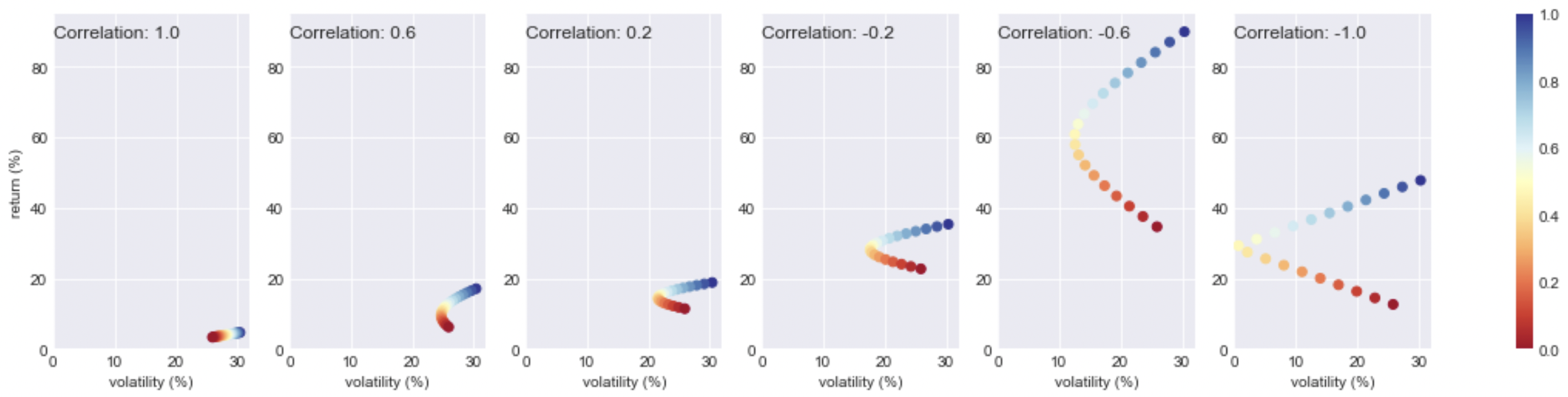
For any given correlation, each point represents the pair return-volatility of a portfolio constructed with some percentage allocation. This can be seen in the colorbar on the right: red corresponds to $\mathbf{w} = (1,0)$, i.e., full allocation of money only to the first stock, whereas blue corresponds to $\mathbf{w} = (0,1)$, i.e., full allocation of money only to the second stock.
We can see that the lower the correlation between the assets, the better the trade-off between return and volatility. In particular, when $\rho=-1$, we could in principle construct a portfolio which guarantees about $30\%$ of annualized return with almost no volatility.