
Understanding and estimating volatility – Quant Finance
25 July 2021In finance, the volatility of an asset is a measure of the variability of its returns. The analytical sophistication of the financial markets has led to an increasingly important role for volatility, for example, in option pricing models.
An important aspect is that it is the variability and not the direction of prices that is relevant. Indeed a certain set of price may be both trending upward or downward but having the same volatility.
Definition
Consider the set of returns of a certain asset, e.g., a stock. Conventionally, the volatility of the stock, denoted here by $\sigma$, is measured as the asset's (annual) standard deviation of returns: $$ \sigma := \sqrt{ \frac{1}{N-1} \sum_{n=1}^N (R_n - \mu)^2 }, $$ where $R_n$ denotes the stock's return at time $t_n$, $\mu$ is the sample mean of the returns, i.e., $$ \mu := \frac{1}{N}\sum_{n=1}^N R_n, $$ and $N$ denotes the number of returns considered. Here, returns are computed using Close prices, hence, this is typically referred to as the Close-to-Close volatility estimator.
Note that the volatility will depend on how many returns $n$ are taken into account and on what kind of returns we have, i.e., daily, monthly, or weekly, and so on. According to this, we will compute either the daily, monthly, or weekly volatility.
Similarly to what we can do with returns, we can annualize the volatility. This is required, in particular, if we need to compare volatilities of different stocks that are obtained from different types of returns.
Suppose we have monthly returns of a stock and we compute the monthly volatility as above. The annualized volatility (or, volatility per year), $\sigma_{y}$, is then a function of the square-root of the time interval on which we first measure it. That is, $$ \sigma_{y} = \sigma_{p} \sqrt{p}, $$ where $\sigma_p$ is the computed (monthly) volatility given the available monthly returns and $p$ denotes the kind of period considered, expressed in days, exactly as for the annualization of returns.
For example:
- In case of daily returns with volatility $\sigma_d$, the annualized volatility is given by $\sigma_{y} = \sigma_d \sqrt{252}$;
- In case of weekly returns with volatility $\sigma_w$, the annualized volatility is given by $\sigma_{y} = \sigma_w \sqrt{52}$;
- In case of monthly returns with volatility $\sigma_m$, the annualized volatility is given by $\sigma_{y} = \sigma_m \sqrt{12}$.
Note that this annualization is indeed justified only if the returns used to compute the volatility are not percentage returns but log-returns, i.e., if $R_t := \log(\frac{P_t}{P_{t-1}})$ (if, for example, we are using daily prices).
This is because it is typically assumed that stock prices are log-normally distributed, which, in turns, implies that log-returns are normally distributed with mean $(\mu - \sigma^2/2)dt$ and variance $\sigma^2 dt$. We have talked about all this stuff in this post.
The key point is the following. Since the variance of the log-returns is $\sigma^2 dt$, for small $dt$, the volatility is then given by $\sigma\sqrt{dt}$. Therefore, one can approximate the volatility for larger period of time by $\sigma\sqrt{T}$, where $\sigma$ is the volatility computed with the available returns.
Understanding the volatility: an example
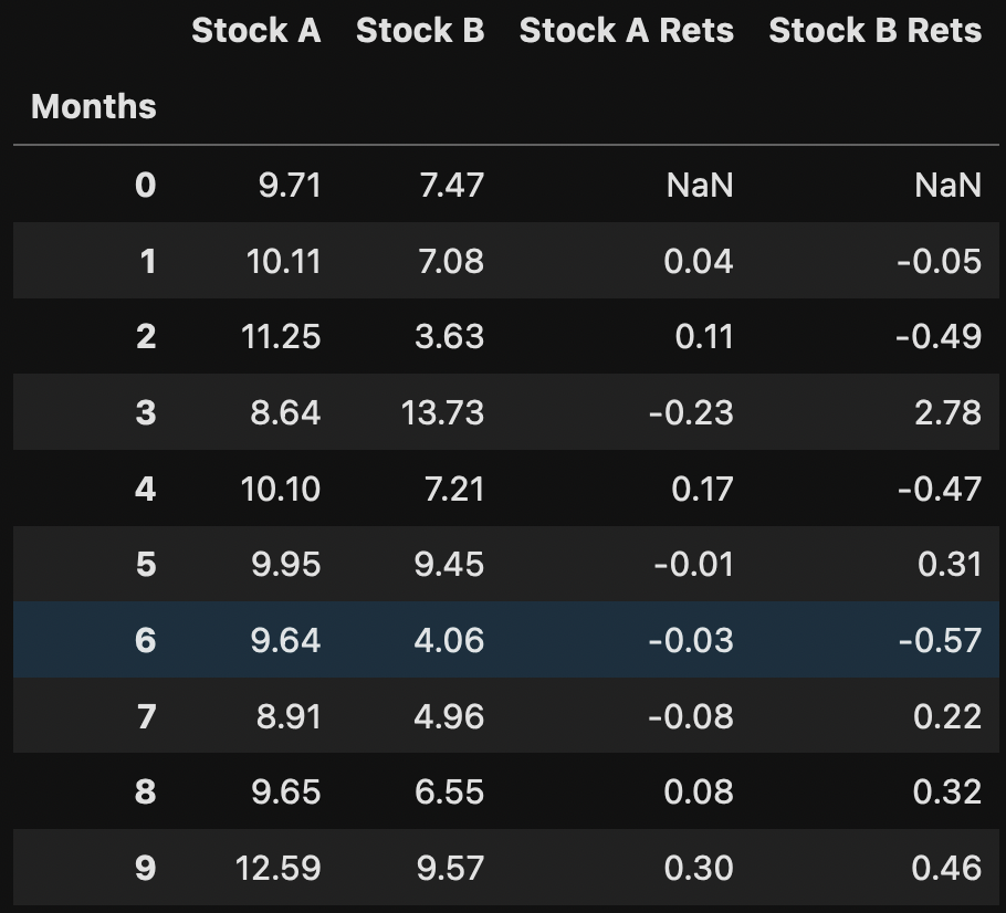
Suppose we have two stocks with the following monthly prices and the corresponding (percentage) returns:
Both the stock prices and the returns look like this:
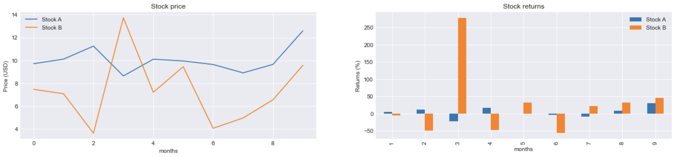
If we compute the total compound return for both stocks at the end of the tenth month we will see that: $$ R^{A}_{cp} = 29.65\% \quad\text{and}\quad R^{B}_{cp} = 28.1\%. $$
Indeed stock A started at 9.71 and on the tenth month its price was 12.59. On the other hand, stock B was worth 7.47 and then its price was 9.57. The (monthly) mean and volatility of the stocks was: $$ \mu_A = 4\% \quad\text{and}\quad \sigma_A = 15\%, $$ for stock A, whereas $$ \mu_B = 27\% \quad\text{and}\quad \sigma_B = 101\%, $$ for stock B. This means that even if the total compound return of the two stocks was about the same (about $30\%$), stock B was almost seven times more volatile than stock A!
Then, if you were to invest in either one of the two stocks, which one would you choose?
Volatility cone
The final volatility that one estimates depends on multiple things, in particular on the number of sessions used. For sure, we know that the volatility does not generally remain constant over time. That is, when we estimate the volatility, we should take into account the fact that it varies in time, hence our estimation should be varying as well.
For example, consider the following total index market returns:
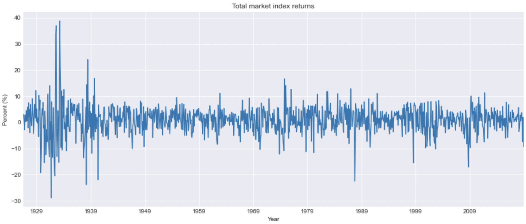
These are monthly returns from July 1926 until December 2018. If we annualize the volatility over the entire period we get $\sigma = 18.35\%$.
However, let us see what happens by computing a trailing (annualized) volatility over 1 year. That is, we pick a rolling window of 12 monthly sessions, we compute the volatility and annualize it. The result is:
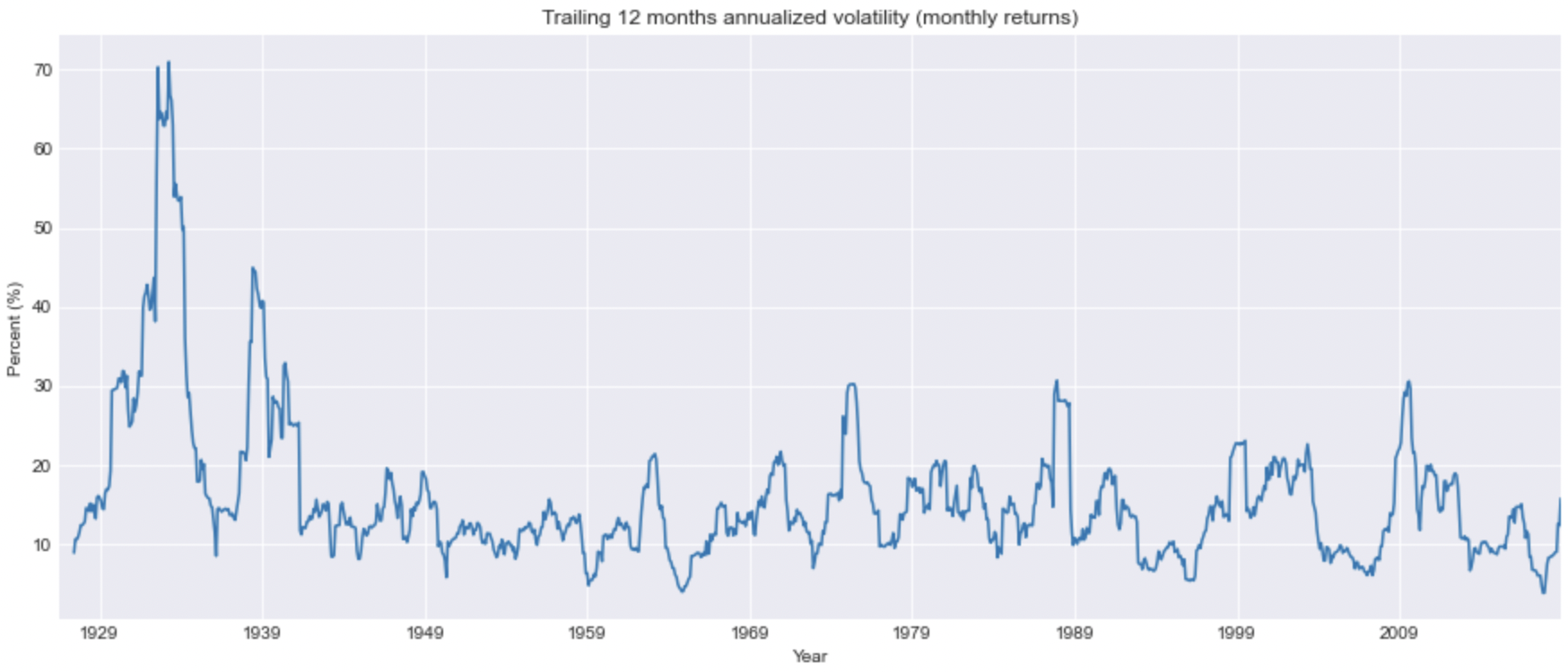
The mean volatility of these trailing volatilities over the entire period is now $\sigma = 15.77\%$.
And if we use a rolling window of 5 years? The result is now the following:
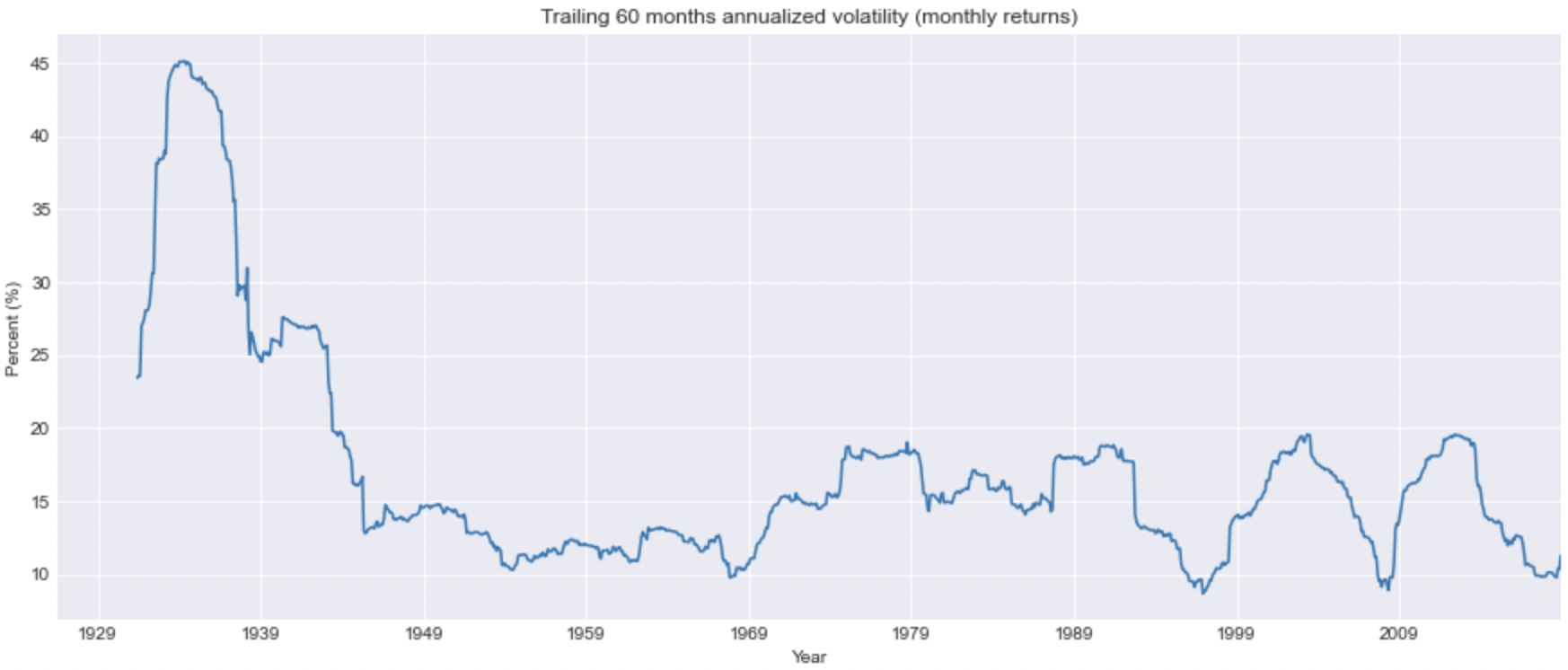
Notice that the entire volatility range decreased. Indeed, we can plot a so called volatility cone and see how the maximum-minimum range of the volatility vary when increasing the rolling windows. We will get something like this:
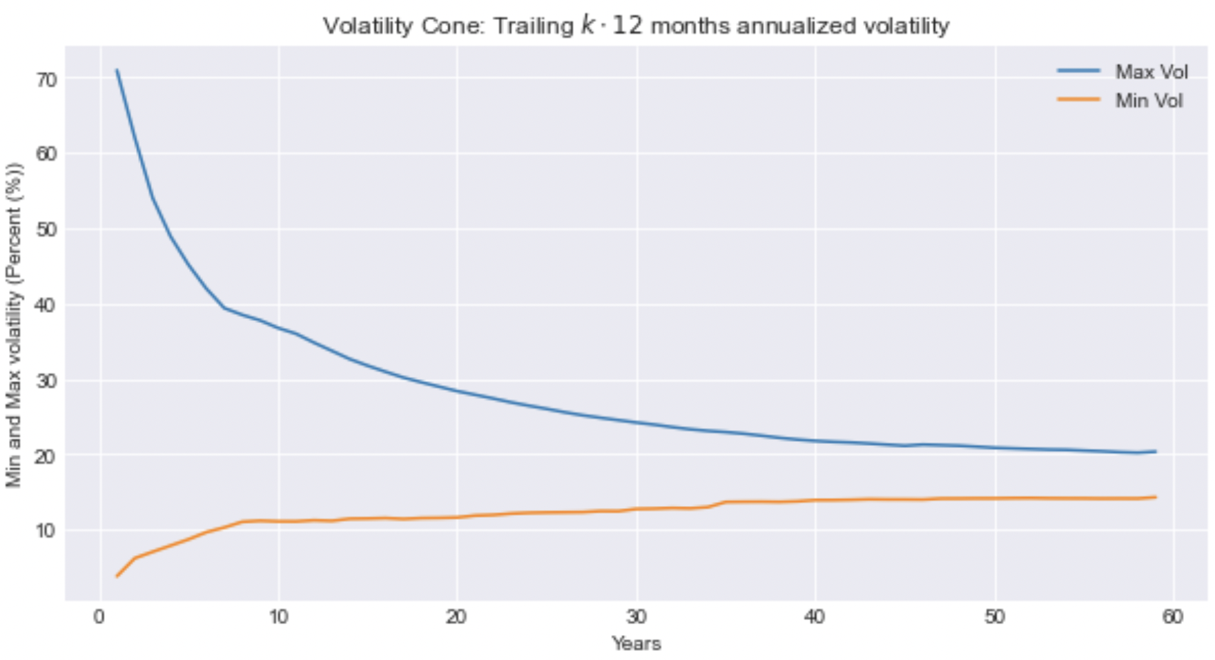
Here, for each year we have a rolling window. Then we can observe how by increasing the window (more sessions for estimating the volatility) the overall range decrease, that is, the cone shrinks.
The assumption that the variance (the square of the volatility) of a series of return may be uniform (constant) is known as homoskedasticity. When this is not the case (basically, always) we talk about heteroskedasticity.
Morevoer, the fact that the variance is not uniform and it is affected by previous variances is referred to as autoregression. We have then to estimate the volatility in a way that takes into account variations over time.
Exponentially Weigthed Moving Average (EWMA)
Let us consider the variance from the definition of the volatility we have given above: $$ \sigma^2 := \frac{1}{N-1} \sum_{n=1}^N (R_n - \mu)^2 = \frac{1}{N-1} \sum_{n=1}^N \varepsilon_n^2 = \frac{1}{N-1} \varepsilon_1^2 + \frac{1}{N-1} \varepsilon_2^2 +\quad ... \quad + \frac{1}{N-1} \varepsilon_N^2, $$ where $\varepsilon_n^2 = (R_n - \mu)^2$ denotes the squared error returns.
By defining the variance (volatility) in this way we are basically computing a weigthed average of the squared error returns, where the weigths are all the same and equal to $1/(N-1)$. That is, we can rewrite: $$ \sigma^2 = \sum_{n=1}^N \alpha_n \varepsilon^2_n \quad\text{where}\quad \alpha_n := \frac{1}{N-1} \quad\text{for all $n$, and}\quad \sum_{n=1}^N \alpha_n = 1. $$ Since $\alpha_n$ are constants, in this way we are considering older returns as much important as more recent ones. This may not make sense since the return distribution is not likely to be stationary and then the volatility will be changing over time. That is, oldest data points are not as informative as the most recent observations.
A better way to proceed is to assign more weight to the most recent observations and less weights to the oldest ones.
This is what the Exponentially Weighted Moving Average (EWMA) does. In this model, we assume that the weights decline exponentially as we move back in time. We define the weigths as: $$ \widehat{\sigma}^2 = \sum_{n=1}^N \widehat{\alpha}_n \epsilon_n^2 \quad\text{where}\quad \widehat{\alpha}_n := \frac{ \lambda^{N-n} }{ \sum_{n=1}^N \lambda^{N-n} } \quad\text{for all $n$}, $$ where $\lambda \in (0,1]$ is called the decay factor.
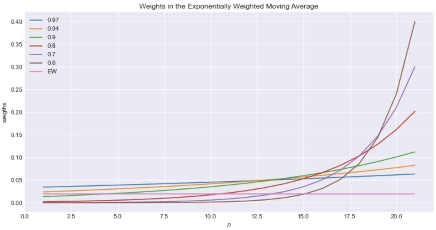
Here, the lowest the decay factor the fastest the decrease of the weigths of oldest returns. Thus, with a very low decay factor, only the very recent returns will significantly impact the volatility. Note that the weights $\widehat{\alpha}_n$ sum to $1$. Also, note that when $\lambda = 1$, then $\widehat{\alpha}_n=1/N$ for all $N$, that is the weights are all constant as in the classic definition of the volatility.
The following plot shows the weigths computed using different decay factors as well as the constant weigths $1/N$ of the definition of the variance:
If we compute the EWMA volatility for the total index market returns we introduced beforehand, we will get:
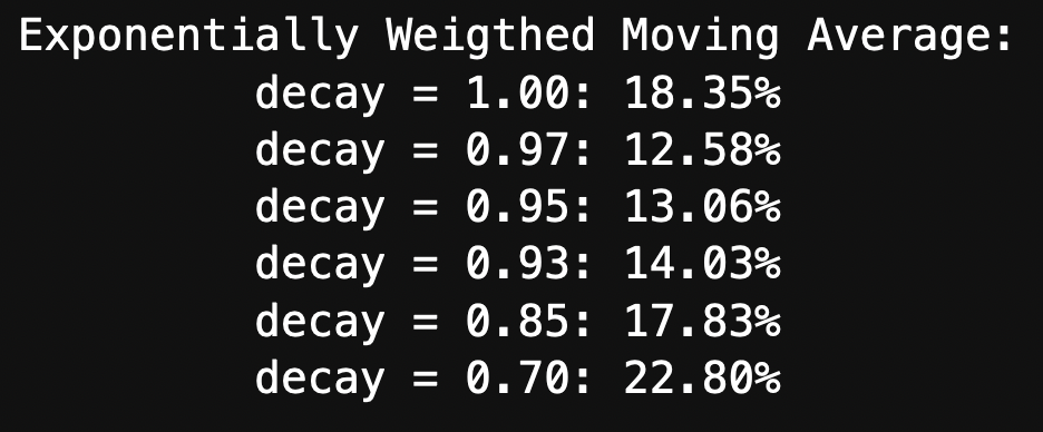
where, notice that for $\lambda=1$ we recover the volatility of $18.35\%$.
A simply python function to compute and annualize the EWMA volatility is the following:
def vol_ewma(r, decay = 0.94, periods_per_year = 12):
    '''
    Computes the annualized EWMA of a series of returns given an input decay factor
    '''
    N = r.shape[0]
    times = np.arange(1,N+1,1)

    # Compute the square error returns
    sq_errs = pd.DataFrame( ( r - r.mean() )**2 )

    # Exponential weights
    weights = [ decay**(N-t) for t in times ] / np.sum(decay**(N-times))
    weights = pd.DataFrame(weights, index=r.index)

    # EWMA volatility
    ewma_vol = (weights * sq_errs).sum()**(0.5)

    # Annualize the computed volatility
    ann_ewma_vol = ewma_vol[0] * np.sqrt(periods_per_year)

    return ann_ewma_vol
Auto-Regressive Conditional Heteroskedasticity(ARCH)
The ARCH model is a variant of the exponential weigthed average idea in which the variance is supposed to be time-varying and dependent on some previous variances.
This model uses a kind of long-term variance estimate as an anchor point. Let us denote by $\bar{\sigma}$ this long-term variance estimator that can be given, for example, by the volatility or the variance estimate over the last 20, 30 years.
We write $ARCH(p)$ to say that we define current (today's) volatility as a function of last previous $p$ squared error returns: $$ \sigma_{N}^2 = \underbrace{ \gamma \bar{\sigma} }_{=:\omega} + \sum_{n=1}^p \alpha_{N-n} \varepsilon_{N-n}^2 \quad \text{where} \quad \gamma + \sum_{n=1}^p \alpha_n = 1. $$ Note that if $p=N$, then we are using the entire set of $N$ returns. On the other hand, if $p=1$, we use only the last previous squared error return: $$ \sigma_{N}^2 = \underbrace{ \gamma \bar{\sigma} }_{=:\omega} + \alpha_{N-1} \varepsilon_{N-1}^2 \quad \text{where} \quad \gamma + \alpha_{N-1} = 1. $$
Generalized Auto-Regressive Conditional Heteroskedasticity (GARCH)
Built on top of the ARCH model, the GARCH model introduces a weighted average of the previous estimates of the variance.
We call by $GARCH(p,q)$ the following model: $$ \sigma_{N}^2 = \underbrace{ \gamma \bar{\sigma} }_{=:\omega} + \sum_{n=1}^p \alpha_{N-n} \varepsilon_{N-n}^2 + \sum_{m=1}^q \beta_{N-m} \sigma_{N-m}^2 \quad \text{where} \quad \gamma + \sum_{n=1}^p \alpha_{N-n} + \sum_{m=1}^q \beta_{N-m} = 1. $$ Note that for $p=q=1$ we have the simplest $GARCH(1,1)$ model: $$ \sigma_{N}^2 = \gamma \bar{\sigma} + \alpha_{N-1} \varepsilon_{N-1}^2 + \beta_{N-1} \sigma^2_{N-1} \quad \text{where} \quad \gamma + \alpha_{N-1} + \beta_{N-1} = 1. $$ Note that when using both the GARCH or the ARCH model we are indeed increasing the number of parameters to estimate since for each asset's volatility we have about $p+q$ or $p$ parameters to estimate, respectively.