
Modern Portfolio Theory - Part 2 – Quant Finance
18 January 2022In the previous post about the Modern Portfolio Theory we have seen how to construct a so called efficient frontier representing the optimal curve of portfolios in the volatility-return plane having the maximum possible return for a certain level of volatility.
Also, we saw an example of the frontier by simulating 20 hypothetical portfolios for a certain set of correlations. In this post, we are going to see an example by using real US stocks but before exploring further let us introduce the following things.
Return-on-Risk (ROR)
The Return-on-Risk (ROR) is a simple quantity which measure how much reward (return) do we get from an investment per unit of risk (volatility). By definition, this is the ratio between the return and the volatility: $$ \text{ROR} := \frac{\text{RETURN}}{\text{RISK}} = \frac{r}{\sigma}, $$ where $r$ is typically the total (compound) return over a certain period under consideration and $\sigma$ denotes the volatility computed over the same period.
Let us compute the RORs for the example with the two stocks introduced here. We had two stocks A and B with about the same (monthly) compound returns $$ r_{A} = 29.65\% \quad\text{and}\quad r_{B} = 28.1\%, $$ but with stock B being almost seven time more volatile than stock A: $$ \sigma_A = 15\% \quad\text{and}\quad \sigma_B = 101\%. $$ The RORs for the stocks are: $$ \text{ROR}_A = \frac{r_{A}}{\sigma_A} = \frac{29.65\%}{15\%} = 1.97 \quad\text{and}\quad \text{ROR}_B = \frac{r_{B}}{\sigma_B} = \frac{28.1\%}{101\%} = 0.27 $$ The higher ROR for stock A says that we get a better return per unit of risk if we invest in it, that is, it is better to invest in stock A rather than stock B although the total compound return of the stocks is about the same.
Sharpe Ratio
The Sharpe Ratio is obtained from adjusting the return in the ROR ratio. The adjustment consists in subtracting the so called risk-free rate from the return. Here, the risk-free rate is nothing but that the return from some asset considered risk-free (for example, US Treasury Bills).
Therefore, $$ \lambda := \frac{E_r}{\sigma} = \frac{r - r_f}{\sigma}, $$ where $E_r$ is called the excess return and $r_f$ is the risk-free rate.
Efficient Frontier example from a real US stocks portfolio
Let us now construct the efficient frontier by using three real US stocks, namely Amazon (AMZN), Coca Cola (KO), and Microsoft (MSFT).
The first step would be to get the stocks prices. We will take the daily prices for a total period from January 2016 up to December 2021. In Python, we can download the prices by using the remote data access provided by pandas_datareader and using Yahoo Finance as source:
from pandas_datareader import data
stocks = pd.DataFrame()
for stock in ["AMZN","KO","MSFT"]:
    # Daily data
    stocks[stock] = data.DataReader(stock,
				    data_source = "yahoo",
				    start       = datetime(2016,1,1),
				    end         = datetime(2022,1,1))["Adj Close"]
This gives:
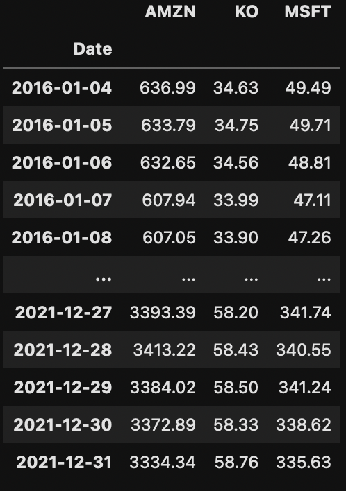
Once we have the stock prices series, we compute the corresponding daily percentage returns:
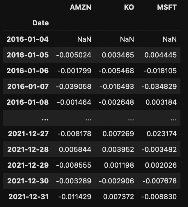
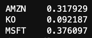
With the series of returns we can compute the annualized return of each stock. Given that we have daily returns, the period considered is $p=252$:
ann_rets = annualize_returns(daily_rets, 252)
Also, given the 3 stocks, we compute the 3-by-3 covariance matrix $\Sigma = [c_{ij}]$ where each element $c_{ij} := \sigma_i \sigma_j \rho_{ij}$, for $i,j=1,\dots,3$, denotes the covariance between assets $i$ and asset $j$, with $\sigma_i$, $\sigma_j$, and $\rho_{ij}$ being the volatilities and the correlation coefficients of assets $i$ and $j$, respectively. For $i=j$, $c_{ii}=\sigma_i^2$ is simply the variance of $i$-th asset. We have:
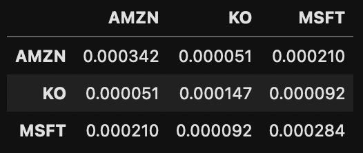
The covariance matrix will be used to compute the portfolio volatility.
Now we simulate 4000 portfolios with the three stocks. In particular, for each portfolio we randomly assign the weigths to the three stocks, $w_1$, $w_2$, and $w_3$, and set $\sum_{i=1}^3 w_i = 1$.
portfolios = pd.DataFrame(columns=["return","volatility","sharpe ratio","w1","w2","w3"])
for i in range(4000):
    # Random weights
    ww = np.random.random(3)
    ww /= np.sum(ww)

    # Annualized portfolio returns
    pret = portfolio_return(ww, ann_rets)

    # Annualized portfolio volatility
    pvol = portfolio_volatility(ww, cov_rets)
    pvol = annualize_vol(pvol, 252)

    # Annualized portfolio Sharpe Ratio
    pspr = sharpe_ratio(pret, 252, risk_free_rate=0, v=pvol)

    # create dataframe
    portfolios = portfolios.append( {"return":pret,
                                     "volatility":pvol,
                                     "sharpe ratio":pspr,
                                     "w1": weights[0],
                                     "w2": weights[1],
                                     "w3": weights[2]},
                                     ignore_index=True)
Similarly to the annualization of returns, annualize_vol is a function which annualizes the volatility. We have seen how here. Furthermore, sharpe_ratio computes the Sharpe Ratio given the annualized portfolio return and volatility and assuming a risk-free rate equal to 0.
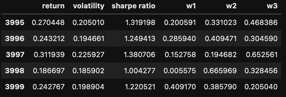
If we look at the last 5 portfolios we have:
Let us finally visualize the portfolios created in the volatility-return plane with a scatter plot coloured by sharpe ratio values.
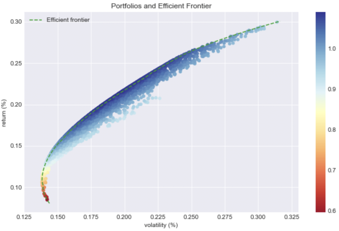
Each dot represents a portfolio whereas the dashed line represents the Efficient Frontier for the portfolio with the 3 stocks we have considered. We can see that if the investor was targeting a return of about 20%, he could simply have hold a portfolio with a volatility of about 18%, even though there are many other portfolios that could 'guarantee' the same return but with higher volatility.
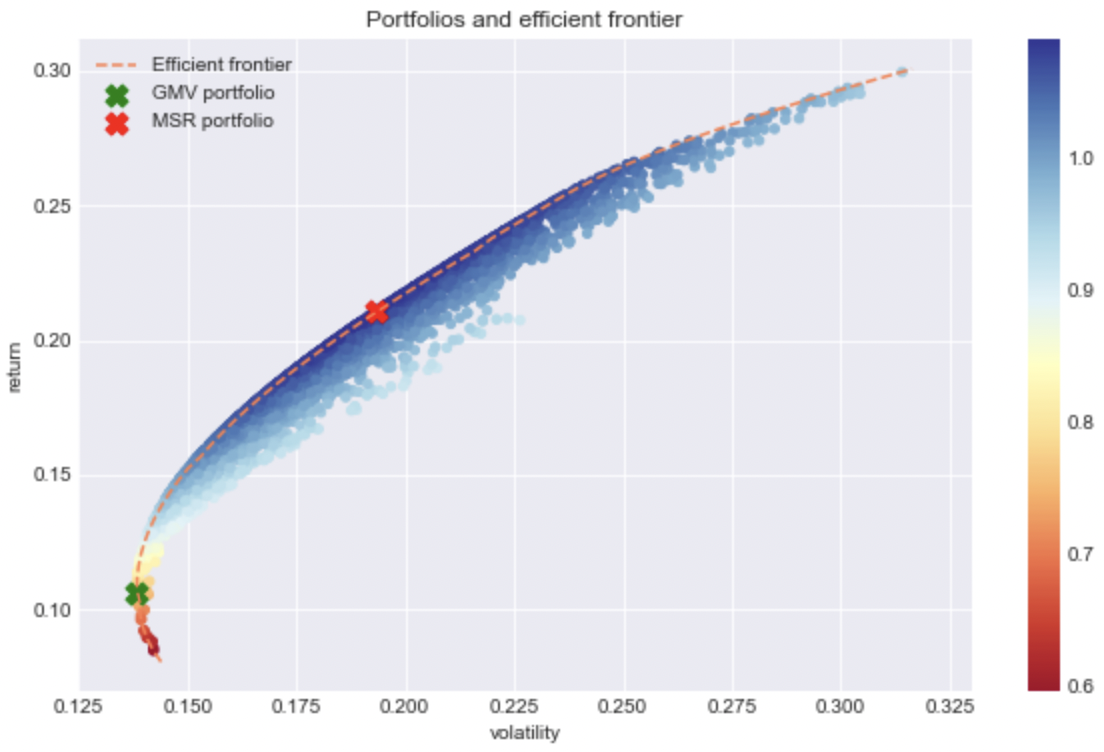
Everything is about carefully choosing the weights of the portfolio. We can see, in particular, that there are two important portfolios:
- the portfolio with the Global Minimum Volatility (GMV);
- the portfolio with the Maximum Sharpe Ratio (MSR).
From the plot, we can easily individuate these two portfolios:
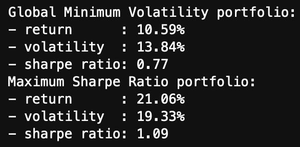
Their returns, volatilities, and Sharpe Ratios are:
Finding the optimal portfolios: a minimization problem
In the examples above, we found the optimal portfolios lying on the efficient frontier by simulating a high number of portfolios. From the plot we could see what the efficient frontier looked like. However, one can directly find the optimal portfolios on the efficient frontier by solving a minimization problem. Then, for example, the scipy optimize method in Python can be used to solve the problem.
Minimizing the volatility
For example, suppose we want to find the portfolio (on the efficient frontier) with the the minimum volatility portfolio (the GMV portfolio). The corresponding minimization problem is: $$ \text{minimize} \;\; \frac{1}{2} \mathbf{w}^T\Sigma\mathbf{w}, $$ subject to $$ \begin{cases} \mathbf{w}^T \mathbf{1} = 1, \\ 0 \leq \mathbf{w} \leq 1. \end{cases} $$ That is, we want to find the weights such that the volatility of the portfolio is minimum, and the weights must be numbers between 0 and 1 that sum up to 1.
If we solve this problem we should find the same GMV portfolio that we found before. If we compare the two results:
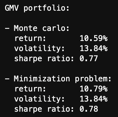
By Monte Carlo we mean the GMV portfolio found by simulating the 4000 portfolios. As we can see the results are pretty similar.
Maximizing the Sharpe Ratio
Likewise, consider now the case of finding the portfolio (on the efficient frontier) with the highest Sharpe Ratio (the MSR portfolio).
This time, we should set a maximization problem, instead of a minimization one. Indeed scipy offers only a minimize method However, this is simply because the maximization of the Sharpe Ratio is nothing but the minimization of the negative Sharpe Ratio.
That is, we have $$ \text{minimize} \;\; - \frac{r_p - r_f}{\sigma_p} $$ subject to $$ \begin{cases} \mathbf{w}^T \mathbf{1} = 1, \\ 0 \leq \mathbf{w} \leq 1. \end{cases} $$
Observation on constraints
It is worth mentioning that so far we have decided to invest all of our capital and, at the same time, our strategy has been long-only. That is, the weights that we allocate to the assets sum to 1 and all of them are positive (because we can only buy the stocks). In particular, these two conditions were imposed when solving the minimization problems.
However, we could in principle not invest all of our capital, which means that we do not necessarily get weights that sum to 1. Furthermore, we may decide to not buy all the stocks. We could also sell some of them.
By short shelling we mean selling an asset that we do not have yet and that we must borrow from someone else.
Short selling with not-normalized weigths: GMV portofolio given a fixed return
We can solve the minimization problem without imposing the constraint on positive weigths and the constraint that the weights sum to $1$. On other hand, let us add the constrain of addressing a fixed target return $r_0$. That is: $$ \text{minimize} \;\; \frac{1}{2} \mathbf{w}^T\Sigma\mathbf{w}, $$ subject to $$ \begin{cases} \mathbf{w}^T \mathbf{R} = R_0, \end{cases} $$ In this case we are allowed to short sell some of the stocks and in principle we do not have to invest all of our capital. Here, $\mathbf{R} = (r_1, r_2, r_3)$ denotes the vector of annualized returns of the three stocks.
For such a problem we can find the analytical solution to by using Lagrange multipliers. We define the Lagrangian of the problem: $$ \mathcal{L}(\mathbf{w}, \lambda) := \frac{1}{2} \mathbf{w}^T\Sigma\mathbf{w} - \lambda( \mathbf{w}^T \mathbf{R} - r_0 ), $$ and put the partial derivatives to zero: $$ \begin{cases} \frac{\partial\mathcal{L}}{\partial \mathbf{w}} &= \frac{1}{2} (2\Sigma \mathbf{w}) - \lambda \mathbf{R} = 0, \\ \frac{\partial\mathcal{L}}{\partial \lambda} &= - \mathbf{w}^T \mathbf{R} + r_0 = 0. \end{cases} $$ From the first equation, we get: $$ \Sigma \mathbf{w} - \lambda \mathbf{R} = 0 \quad\Longrightarrow\quad \mathbf{w} = \lambda \Sigma^{-1}\mathbf{R}, $$ and inserting into the second equation: $$ - ( \lambda \Sigma^{-1}\mathbf{R} )^T \mathbf{R} + R_0 = 0 \quad\Longrightarrow\quad \lambda \mathbf{R}^T \Sigma^{-1} \mathbf{R} = R_0 \quad\Longrightarrow\quad \lambda = \frac{R_0}{\mathbf{R}^T \Sigma^{-1} \mathbf{R}}. $$ Note that since $\Sigma$ was symmetric, so is $\Sigma^{-1}$, from which $(\Sigma^{-1})^T = \Sigma^{-1}$. We can then insert $\lambda$ back into the first equation and obtain: $$ \mathbf{w}^* = R_0 \frac{\Sigma^{-1}\mathbf{R}}{\mathbf{R}^T \Sigma^{-1} \mathbf{R}}, $$ which is therefore the analytical expression for the weights. Notice that since we have not imposed the constraint on the normalisation, we are not guaranteed that such vector of weights sum to $1$.
Short selling with normalized weigths: GMV portofolio given a fixed return
Analogously, we can also also find the analytical expression for optimal weights in case we add the condition that they sum to $1$, but without requiring that they are all positive, i.e.: $$ \text{minimize} \;\; \frac{1}{2} \mathbf{w}^T\Sigma\mathbf{w}, $$ subject to $$ \begin{cases} \mathbf{w}^T \mathbf{R} &= R_0, \\ \mathbf{w}^T \mathbf{1} &= 1. \end{cases} $$ This is again the case in which we can short sell the stocks but this time we invest all of the capital.
We define the Lagrangian: $$ \mathcal{L}(\mathbf{w}, \lambda) := \frac{1}{2} \mathbf{w}^T\Sigma\mathbf{w} - \lambda( \mathbf{w}^T \mathbf{R} - R_0) - \delta(\mathbf{w}^T\mathbf{1}-1), $$ and put the partial derivatives to zero: $$ \begin{cases} \frac{\partial\mathcal{L}}{\partial \mathbf{w}} &= \frac{1}{2} (2\Sigma \mathbf{w}) - \lambda \mathbf{R} - \delta \mathbf{1}= 0, \\ \frac{\partial\mathcal{L}}{\partial \lambda} &= - \mathbf{w}^T \mathbf{R} + R_0 = 0, \\ \frac{\partial\mathcal{L}}{\partial \lambda} &= - \mathbf{w}^T \mathbf{1} + R_0 = 0. \end{cases} $$ From the first equation we get: $$ \mathbf{w} = \Sigma^{-1}(\lambda \mathbf{R} + \delta\mathbf{1}), $$ and we can insert it into the second and the third equation, respectively: \begin{cases} \left(\Sigma^{-1}(\lambda \mathbf{R} + \delta\mathbf{1}) \right)^T\mathbf{R} &= \lambda \mathbf{R}^T\Sigma^{-1}\mathbf{R} + \delta\mathbf{1}\Sigma^{-1}\mathbf{R} = R_0, \\ \left(\Sigma^{-1}(\lambda \mathbf{R} + \delta\mathbf{1}) \right)^T\mathbf{1} &= \lambda \mathbf{R}^T\Sigma^{-1}\mathbf{1} + \delta\mathbf{1}\Sigma^{-1}\mathbf{1} = 1. \end{cases} Let us define the following fixed numbers: $$ \begin{cases} A & := \mathbf{R}^T \Sigma^{-1} \mathbf{R}, \\ B & := \mathbf{1}^T \Sigma^{-1} \mathbf{R} \equiv \mathbf{R}^T \Sigma^{-1} \mathbf{1}, \\ C & := \mathbf{1}^T \Sigma^{-1} \mathbf{1}, \end{cases} $$ where notice that in B the second equation is true since $\Sigma^{-1}$ is a symmetric matrix. Hence we have the following system to solve: $$ \begin{cases} \lambda A + \delta B &= R_0, \\ \lambda B + \delta C &= 1. \end{cases} $$ From the second equation we find $\lambda$ and put it into the first equation: $$ \lambda = \frac{1-\delta C}{B} \quad\Longrightarrow\quad \frac{1-\delta C}{B} A + \delta B = R_0 \quad\text{from which}\quad \delta = \frac{R_0B - A}{B^2-AC}. $$ Now, we put $\delta$ back into $\lambda$: $$ \lambda = \frac{1 - \frac{R_0 B-A}{B^2-AC}C }{B} = \frac{B - R_0 C}{B^2-AC}. $$ Finally, we can put both $\lambda$ and $\delta$ we have just find back into $\mathbf{w}$ and find the optimal weights: \begin{equation} \begin{split} \mathbf{w}^* = \lambda \Sigma^{-1} \mathbf{R} + \delta \Sigma^{-1} \mathbf{1} & = \frac{B - R_0 C}{B^2-AC} \Sigma^{-1} \mathbf{R} + \frac{R_0B - A}{B^2-AC} \Sigma^{-1}\mathbf{1} \\ &= \frac{1}{B^2-AC}\left(B\Sigma^{-1}\mathbf{R} - A\Sigma^{-1}\mathbf{1} \right) + R_0 \Bigl( \frac{1}{B^2-AC}\left(B\Sigma^{-1}\mathbf{1} - C\Sigma^{-1}\mathbf{R} \right) \Bigr). \end{split} \end{equation}